
Notice to the reader: That is the fourth in a sequence of articles I am publishing right here taken from my e-book, “Investing with the Pattern.” Hopefully, you will see this content material helpful. Market myths are usually perpetuated by repetition, deceptive symbolic connections, and the whole ignorance of details. The world of finance is stuffed with such tendencies, and right here, you will see some examples. Please remember that not all of those examples are completely deceptive — they’re generally legitimate — however have too many holes in them to be worthwhile as funding ideas. And never all are instantly associated to investing and finance. Take pleasure in! – Greg
Threat and Uncertainty
Is volatility danger? (Right here we go once more.)
Within the sterile laboratory of recent finance, danger is outlined by volatility as measured by customary deviation. Nevertheless, that assumes the vary of outcomes is a traditional distribution (bell curve). Not often do the markets yield to regular.
When an investor opens his or her brokerage assertion, it reveals the next portfolio knowledge for the final yr:
- Commonplace Deviation = .65
- Loss for the 12 months =.35 p.c
Which one do you assume will catch their consideration? I severely doubt any investor goes to name his or her advisor and complain about a normal deviation of .65. Nevertheless, the .35 p.c loss will get their consideration. Even traders who haven’t any information of finance or investments know what danger is—it’s the lack of capital.
Threat is just not volatility; it’s drawdown (lack of capital). Nevertheless, within the quick time period, volatility is an efficient proxy for danger, however over the long run, drawdown is a a lot better measure of danger. Volatility does contribute to danger, however it additionally contributes to market positive aspects.
Threat and uncertainty are not the identical factor.
Threat will be measured. Uncertainty can’t be measured.
A jar comprises 5 purple balls and 5 blue balls. Within the previous days we referred to as it an urn as an alternative of a jar. Blindly pick a ball. What are the percentages of selecting a purple ball? There are 5 purple balls and the overall variety of balls is 10. Subsequently the percentages of selecting a purple ball are 5/10 =.5 or 50 p.c.
That’s Threat! It may be calculated.
Suppose you weren’t advised the variety of purple or blue balls within the jar. What are the percentages of selecting a purple ball? That’s Uncertainty!
 Determine 3.8
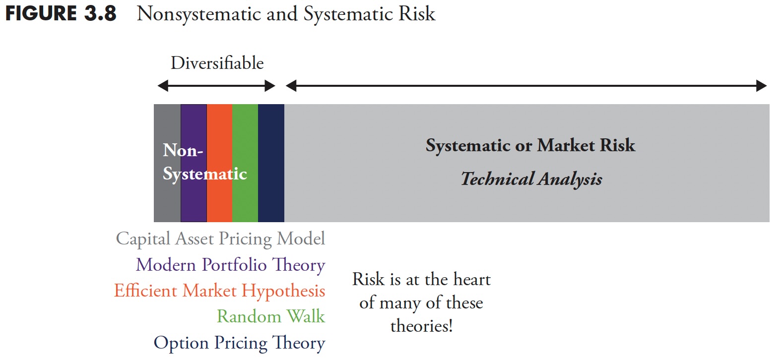
Determine 3.8 is an try to visualise how fashionable finance is concentrated on danger, however have you ever ever questioned or considered which aspect of danger they take care of? Truly they do an awesome job of analyzing danger; danger is on the coronary heart of all of the theories of Fashionable Portfolio Idea (Capital Asset Pricing Mannequin, Environment friendly Market Speculation, Random Stroll, Possibility Pricing Idea, and so forth.). The danger that they try to discourage.mine is called nonsystematic danger, or you’ll have heard it as diversifiable danger. Diversification is a free lunch and may by no means be ignored. The world of fi nance is concentrated on diversifiable or nonsystematic danger. Nevertheless, there’s a a lot bigger piece of the chance pie, and that’s referred to as systematic danger. Upon getting adequately diversified, then it appears that you’re solely coping with systematic danger. Systematic danger is what technical evaluation makes an attempt to take care of. It’s also generally known as drawdown, lack of capital, and in sure conditions as a bear market.
Again to the Unique Query: Is Volatility Threat?
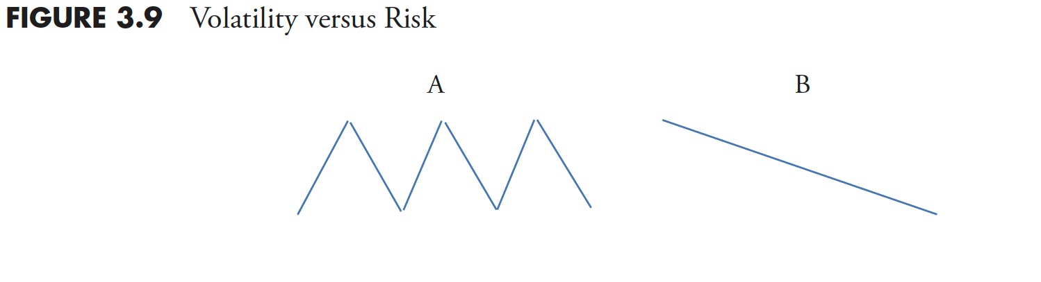
Two easy worth actions are proven in Determine 3.9 ; which represents extra danger, instance A or instance B?
 Determine 3.9
Fashionable finance would have you ever consider that A is riskier due to its volatility. Nevertheless, you possibly can discover from this overly easy instance that the worth ended up precisely the place it started; subsequently, you didn’t earn cash or lose cash. B, based mostly on the idea of volatility as danger, has no danger in keeping with principle; nonetheless, you misplaced cash within the course of. I feel it’s apparent which is danger and which is barely principle.
Is Linear Evaluation Good Sufficient?
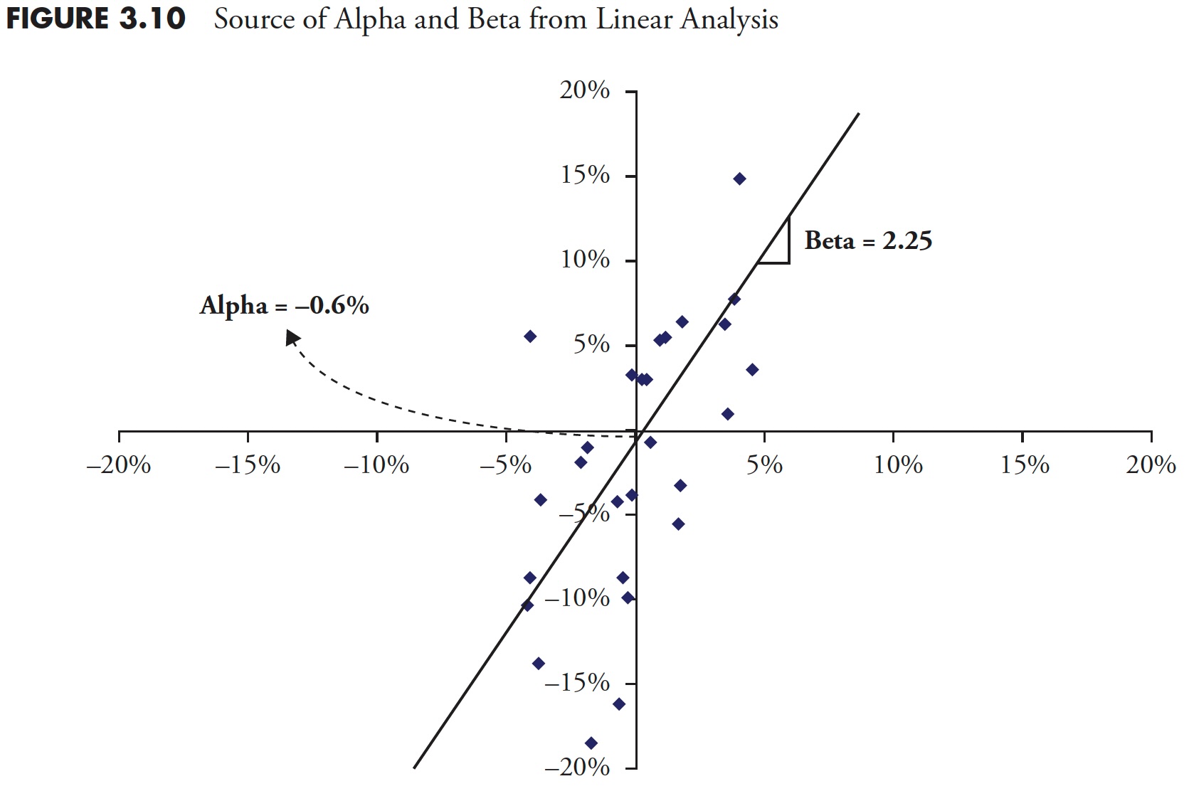
Determine 3.10 is called a Cartesian coordinate system, generally known as a scatter diagram, used typically to check two points and derive relationships between them. The returns of 1 are plotted on the X-axis (abscissa/horizontal) and the returns of the opposite are plotted utilizing the Y-axis (ordinate/vertical). These small diamonds are the information factors. An idea generally known as regression is then utilized by calculating a least-squares match of the information factors. That is the straight line that you simply see beneath. Then, a little bit highschool geometry is used on the equation for a straight line, which is y=mx+b, the place m is the slope of the road and b is the the place the road crosses the Y axis (a.ok.a. the y–intercept). So upon getting the linearly fitted line, you possibly can measure the slope and y–intercept, and this provides you with the beta (slope) and alpha (y-intercept).
 Determine 3.10
The next statistical parts can all be derived from easy linear evaluation.
- Uncooked Beta
- Alpha
- R^2 (Coefficient of Dedication)
- R (Correlation)
- Commonplace Deviation of Error
- Commonplace Error of Alpha
- Commonplace Error of Beta
- t-Take a look at
- Significance
- Final T-Worth
- Final P-Worth
Linear Regression Should Have Correlation
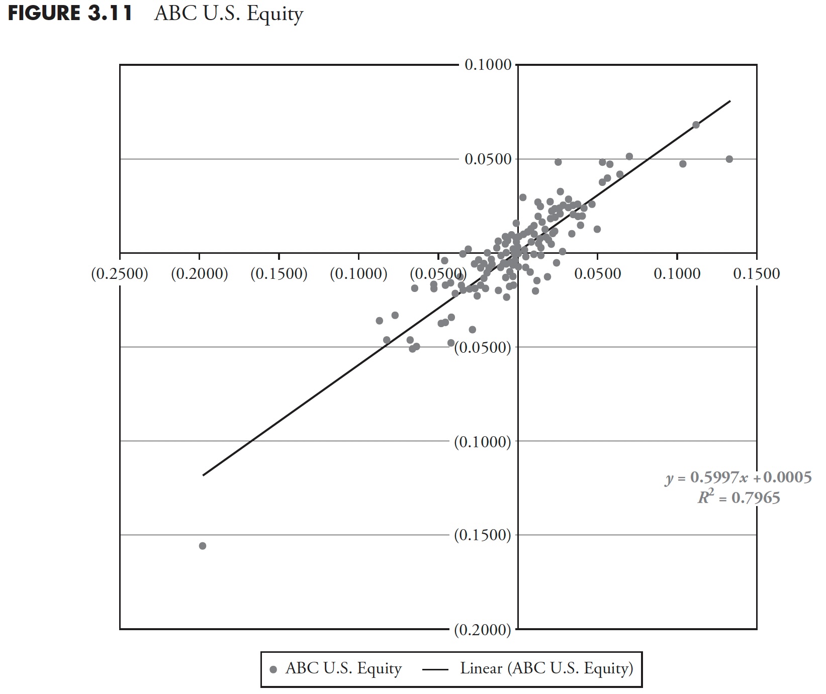
Determine 3.11 is a scatter plot of a fictional fund ABC (Y-axis) plotted in opposition to the S&P 500 (X-axis).
 Determine 3.11
The least-squared regression line is plotted and the equation is proven as:
Y = 0.5997x + 0.0005, which suggests the slope is .5997 and the y-intercept is 0.0005.
A slope of 1.0 would imply that the Beta of the fund was the identical in comparison with the index, and the road on the plot can be a quadrant bisector (if the plot have been a sq., the road can be shifting up and to the proper at 45 levels). So, a slope of 0.5997 means the fund has a decrease beta than the index. The y-intercept is a optimistic quantity, though barely, however which means the fund outperformed the index.
R^2 is the Coefficient of Dedication, also called the goodness of match. Now, I perceive that coping with optimistic numbers has some benefits, however, generally, R^2 can also be lowering the quantity of data. Let me clarify. We all know that R is correlation, the statistical measure that reveals the connection between two datasets and the way intently they’re aligned. That isn’t the textbook reply for correlation, however will suffice for now. Correlation ranges from +1 (completely correlated) to -1 (inversely correlated), with 0 being non-correlated. Good data to know; is the fund correlated to the market, inversely correlated to the market, or not correlated in any respect? Squaring correlation provides you with an all the time optimistic quantity (keep in mind least squares?), however why take away the details about the extent of correlation? R^2 is not going to inform you whether it is correlated or inversely correlated. Truly, I feel it’s the social science’s concern of destructive numbers. Nevertheless, in equity, R^2 will present the p.c dependency of 1 variable over the opposite—in principle.
The R^2 in Determine 3.11 is 0.7965, which suggests there’s a truthful diploma of correlation, we simply do not know whether it is optimistic correlation or inverse correlation. To get correlation, merely take the sq. root of 0.7965 to get R=0.8924684 (sure, an try at humor), which suggests R is also -0.8924684. Anyway, hopefully you get my level.
Lastly, discover how the information factors are all clustered pretty intently to the least squares line, which visually reveals you that this fund is pretty well-correlated to the index.
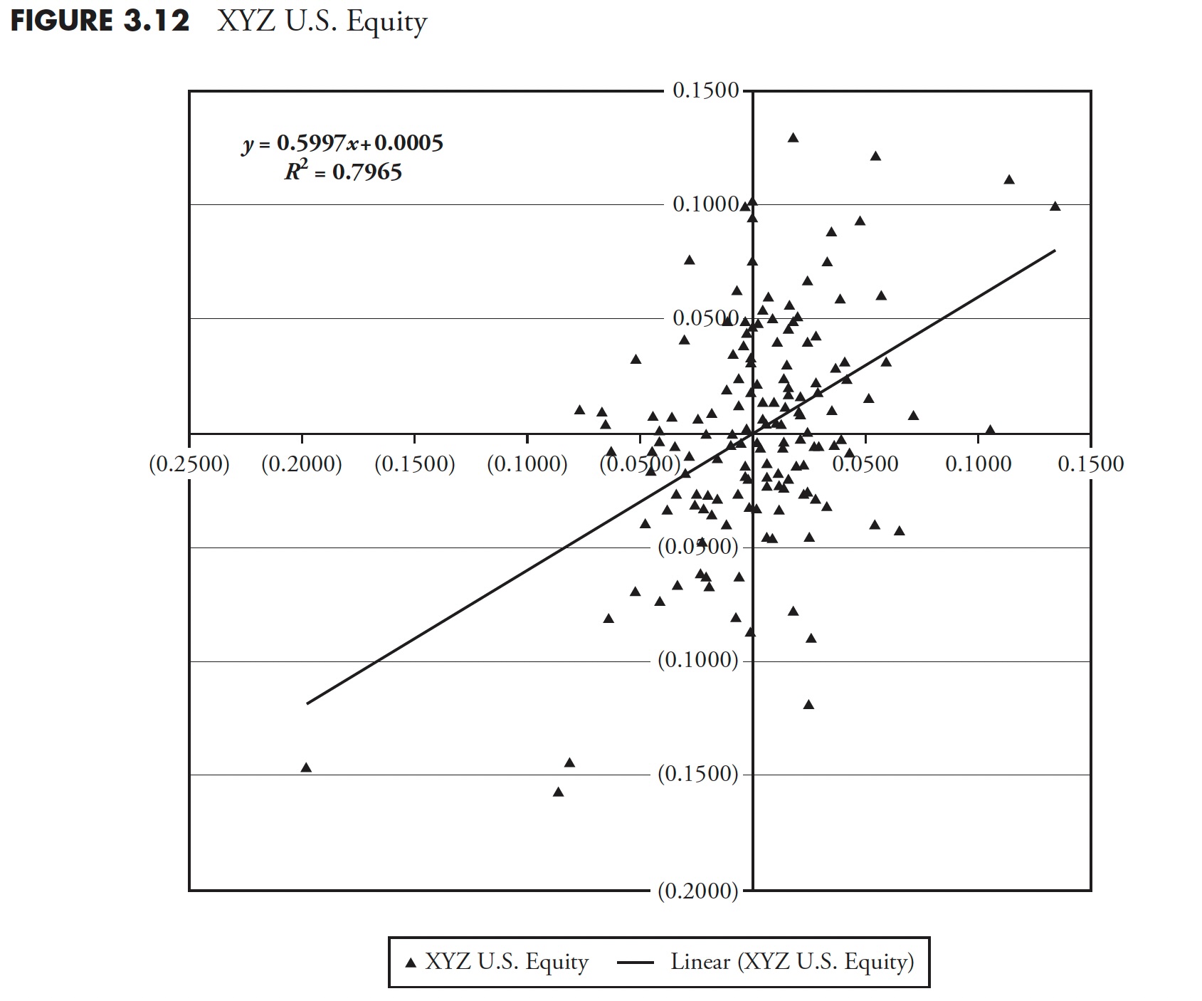
Determine 3.12 reveals fund XYZ plotted in opposition to an index. Discover that the linear least-squared match equation (y = 0.5997x + 0.0005) is strictly the identical because the earlier instance. Nevertheless the worth of R^2 is 0.2051, which is significantly totally different than the earlier instance. Visually, you possibly can see that the information factors are extra scattered than within the earlier instance, so, simply based mostly on the visible commentary, you understand this fund is just not almost as correlated because the earlier fund ABC. But we discover that the least squares regression line is oriented precisely the identical, so the values of alpha and beta are the identical for this fund (XYZ) as they have been for fund (ABC) above.
 Determine 3.12
So what is the distinction, you’re hopefully asking? The distinction is that one fund is just not almost as correlated as the opposite. We all know that they’re each positively correlated from visible examination, however except the worth of R (correlation) is proven, we do not know any extra in regards to the correlation. This is without doubt one of the horrible shortcomings of such a evaluation. Right here is the message: if it is not correlated, then the values derived for alpha and beta are completely meaningless. But I see publications rating funds and exhibiting R^2, alpha, and beta, however by no means a point out of R. Disgrace on them!
 Determine 3.13
The scatterplot in Determine 3.13 reveals each funds plotted with the index. You’ll be able to clearly see that fund XYZ (triangles) is just not almost as correlated as fund ABC (circles). But the linear statistics of recent finance doesn’t delineate a distinction between the 2. My solely remark to them is: Keep out of aviation.
The 60/40 Fantasy Uncovered
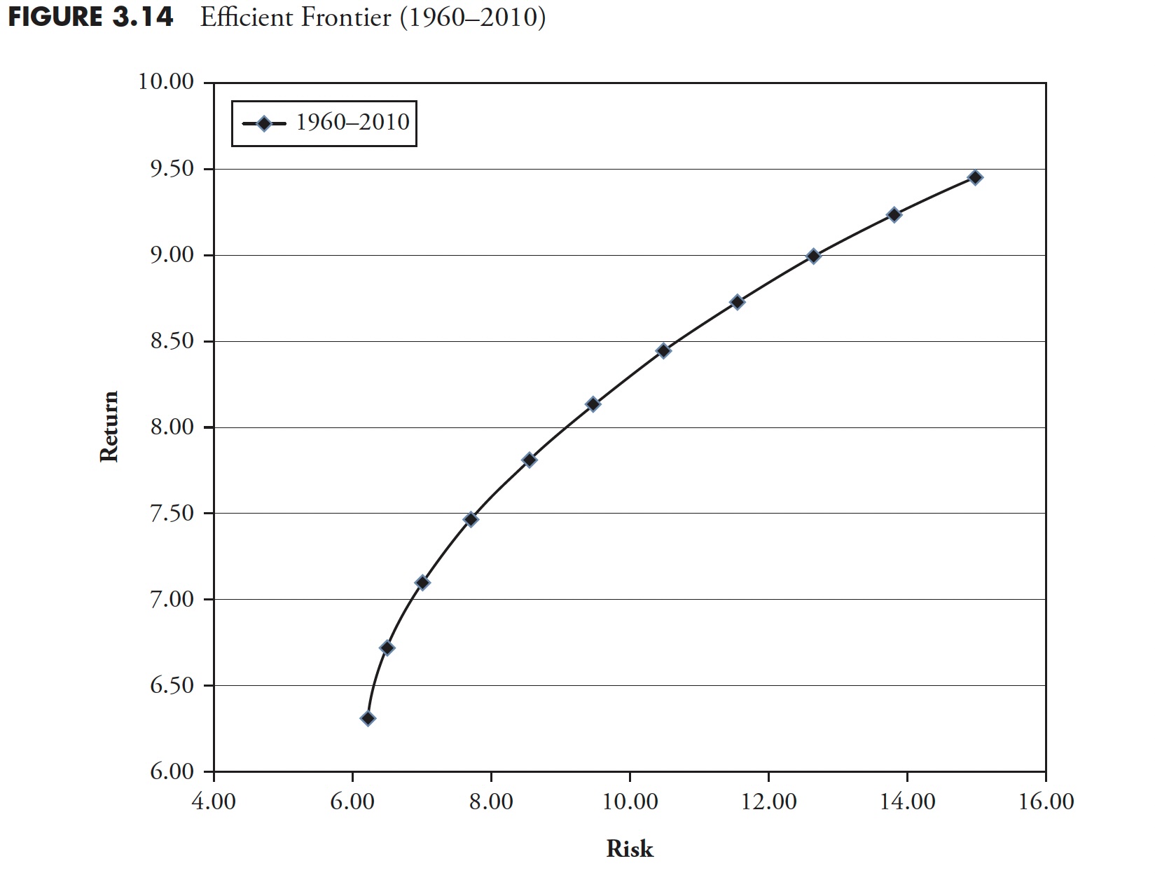
It’s nearly unattainable to see any efficiency comparisons that not solely present a benchmark, but in addition a mixture of 60% fairness and 40% mounted revenue, generally known as 60/40 within the fund trade. The environment friendly frontier is a type of phrases that got here from a principle developed a long time in the past on danger administration. Fashionable finance seems at a plot of returns versus danger, and, in fact, by danger, it means customary deviation. That is the primary mistake made with this idea. Then it plots quite a lot of totally different asset lessons on the identical plot and derives the environment friendly frontier, which reveals you the extent of danger you’re taking for the asset lessons you need to put money into. Determine 3.14 reveals the environment friendly frontier curve from 1960 to 2010 (an intermediate bond part was used).
Subsequent, if you happen to draw a line that’s tangent with the curve and have it cross the vertical return axis on the degree for assumed danger free, then the purpose of tangential is the correct mixture of fairness and bonds. I didn’t try to do that right here, because the willpower of the chance free fee to make use of over a 50-year interval presents an excessive amount of subjectivity. From 1960 to current, that blend of shares and bonds is about 60/40.
 Determine 3.14
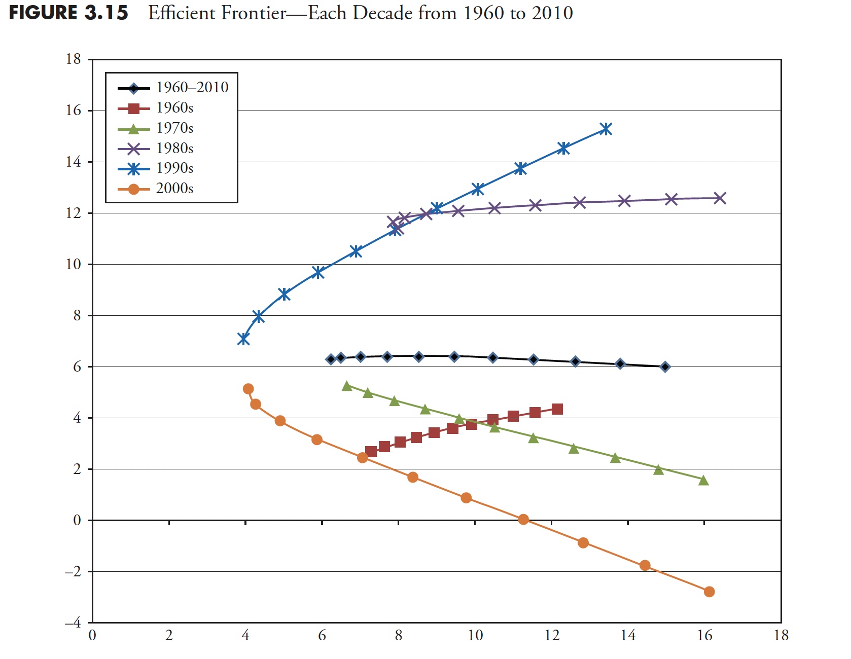
The ever-present 60/40 ratio of shares to bonds, which reveals up in most efficiency comparisons, gleans the message that, for over 50 years of information, nothing has modified. Does anybody truly consider that? Determine 3.15 is a chart exhibiting the environment friendly frontier for every particular person decade within the 1960 to 2010 interval. Clearly, every decade has its personal environment friendly frontier and its correct mixture of fairness and bonds. But the world of finance nonetheless sticks to the customarily mistaken mixture of 60/40. It might very effectively be a great mixture of property, however the knowledge says it’s dynamic and ought to be reviewed on a periodic foundation. Discover that the a long time of 1970 and 2000 confirmed comparable downward curves, which means that shares weren’t almost nearly as good as bonds. Conversely the a long time of 1980 and 1990 have been the other.
 Determine 3.15
In an interview with Jason Zweig on October 15, 2004, Peter Bernstein mentioned {that a} inflexible allocation coverage like 60/40 is one other means of passing the buck and avoiding selections. Did you need to be 40 p.c invested in bonds through the Nineteen Seventies when rates of interest soared? Did you need to solely be invested 60 p.c in equities within the interval from 1982 to 2000, which was the best bull market in historical past? After all not! Markets are dynamic, and funding methods ought to be too. Lastly, some evaluation will present {that a} 60/40 portfolio is extremely correlated to an all-equity portfolio.
Discounted Money Movement Mannequin
When finding out fashionable finance, and after years of listening to in regards to the discounted money circulation (DCF) mannequin, I’ve this to say in regards to the discounted money circulation mannequin. Initially, you will need to resolve on six values in regards to the future. They’re proven beneath. You probably have learn this e-book this far, you in all probability know what’s coming subsequent.
Low cost Price
- Price of Fairness, in valuing fairness
- Price of Capital, in valuing the agency
Money Flows
- Money Flows to Fairness
- Money Flows to Agency
Progress (to get future money flows)
- Progress in Fairness Earnings
- Progress in Agency Earnings (Working Revenue)
The inputs (above) to the DCF course of should all be appropriate or the mannequin fails fully. The percentages of efficiently developing with appropriate (guesses) inputs are extraordinarily low, but that is utilized in fashionable finance routinely. This jogs my memory of the Kenneth Arrow story on forecasting in Chapter 5. When requested in regards to the discounted money circulation mannequin, I liken it to the Hubble Telescope; transfer it an inch and swiftly you’re looking at a special galaxy.
The objective of this chapter, on the very minimal, is to trigger you to problem what fashionable finance has supplied. I apologize for beating some ideas with a stick, however generally a number of approaches to point out one thing are higher within the hope that one will stay with the reader. There was sufficient math to scare the typical individual; Half 4 focuses on the vast use of the time period common. The objective is to point out that utilizing long-term averages will be completely inappropriate for many traders.
Thanks for studying this far. I intend to publish one article on this sequence each week. Cannot wait? The e-book is on the market right here.

