
Picture by Writer
In case you can add just one talent—and inarguably crucial—to your information science toolbox, it’s SQL. Within the Python information evaluation ecosystem, nevertheless, pandas is a strong and standard library.
However, in case you are new to pandas, studying your means round pandas features—for grouping, aggregation, joins, and extra—could be overwhelming. It could be a lot simpler to question your dataframes with SQL as an alternative. The pandasql library allows you to just do that!
So let’s learn to use the pandasql library to run SQL queries on a pandas dataframe on a pattern dataset.
Earlier than we go any additional, let’s arrange our working surroundings.
Putting in pandasql
In case you’re utilizing Google Colab, you may set up pandasql utilizing `pip` and code alongside:
In case you’re utilizing Python in your native machine, guarantee that you’ve got pandas and Seaborn put in in a devoted digital surroundings for this undertaking. You should utilize the built-in venv bundle to create and handle digital environments.
I’m operating Python 3.11 on Ubuntu LTS 22.04. So the next directions are for Ubuntu (also needs to work on a Mac). In case you’re on a Home windows machine, comply with these directions to create and activate digital environments.
To create a digital surroundings (v1 right here), run the next command in your undertaking listing:
Then activate the digital surroundings:
Now set up pandas, seaborn, and pandasql:
pip3 set up pandas seaborn pandasql
Observe: In case you don’t have already got `pip` put in, you may replace the system packages and set up it by operating: apt set up python3-pip.
The `sqldf` Perform
To run SQL queries on a pandas dataframe, you may import and use sqldf with the next syntax:
from pandasql import sqldf
sqldf(question, globals())
Right here,
questionrepresents the SQL question that you simply need to execute on the pandas dataframe. It must be a string containing a sound SQL question.globals()specifies the worldwide namespace the place the dataframe(s) used within the question are outlined.
Let’s begin by importing the required packages and the sqldf perform from pandasql:
import pandas as pd
import seaborn as sns
from pandasql import sqldf
As a result of we’ll run a number of queries on the dataframe, we will outline a perform so we will name it by passing within the question because the argument:
# Outline a reusable perform for operating SQL queries
run_query = lambda question: sqldf(question, globals())
For all of the examples that comply with, we’ll run the run_query perform (that makes use of sqldf() underneath the hood) to execute the SQL question on the tips_df dataframe. We’ll then print out the returned end result.
Loading the Dataset
For this tutorial, we’ll use the “ideas” dataset constructed into the Seaborn library. The “ideas” dataset incorporates details about restaurant ideas, together with the full invoice, tip quantity, gender of the payer, day of the week, and extra.
Lload the “tip” dataset into the dataframe tips_df:
# Load the "ideas" dataset right into a pandas dataframe
tips_df = sns.load_dataset("ideas")
Instance 1 – Deciding on Information
Right here’s our first question—a easy SELECT assertion:
# Easy choose question
query_1 = """
SELECT *
FROM tips_df
LIMIT 10;
"""
result_1 = run_query(query_1)
print(result_1)
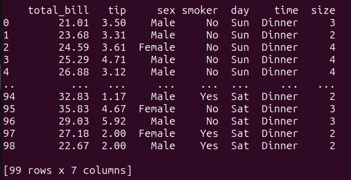
As seen, this question selects all the columns from the tips_df dataframe, and limits the output to the primary 10 rows utilizing the `LIMIT` key phrase. It’s equal to performing tips_df.head(10) in pandas:
Output of query_1
Instance 2 – Filtering Primarily based on a Situation
Subsequent, let’s write a question to filter the outcomes primarily based on circumstances:
# filtering primarily based on a situation
query_2 = """
SELECT *
FROM tips_df
WHERE total_bill > 30 AND tip > 5;
"""

result_2 = run_query(query_2)
print(result_2)
This question filters the tips_df dataframe primarily based on the situation specified within the WHERE clause. It selects all columns from the tips_df dataframe the place the ‘total_bill’ is larger than 30 and the ‘tip’ quantity is larger than 5.
Working query_2 offers the next end result:
Output of query_2
Instance 3 – Grouping and Aggregation
Let’s run the next question to get the common invoice quantity grouped by the day:
# grouping and aggregation
query_3 = """
SELECT day, AVG(total_bill) as avg_bill
FROM tips_df
GROUP BY day;
"""

result_3 = run_query(query_3)
print(result_3)
Right here’s the output:
Output of query_3
We see that the common invoice quantity on weekends is marginally larger.
Let’s take one other instance for grouping and aggregations. Think about the next question:
query_4 = """
SELECT day, COUNT(*) as num_transactions, AVG(total_bill) as avg_bill, MAX(tip) as max_tip
FROM tips_df
GROUP BY day;
"""

result_4 = run_query(query_4)
print(result_4)
The question query_4 teams the info within the tips_df dataframe by the ‘day’ column and calculates the next combination features for every group:
num_transactions: the rely of transactions,avg_bill: the common of the ‘total_bill’ column, andmax_tip: the utmost worth of the ‘tip’ column.
As seen, we get the above portions grouped by the day:
Output of query_4
Instance 4 – Subqueries
Let’s add an instance question that makes use of a subquery:
# subqueries
query_5 = """
SELECT *
FROM tips_df
WHERE total_bill > (SELECT AVG(total_bill) FROM tips_df);
"""

result_5 = run_query(query_5)
print(result_5)
Right here,
- The interior subquery calculates the common worth of the ‘total_bill’ column from the
tips_dfdataframe. - The outer question then selects all columns from the
tips_dfdataframe the place the ‘total_bill’ is larger than the calculated common worth.
Working query_5 offers the next:
Output of query_5
Instance 5 – Becoming a member of Two DataFrames
We solely have one dataframe. To carry out a easy be a part of, let’s create one other dataframe like so:
# Create one other DataFrame to affix with tips_df
other_data = pd.DataFrame({
    'day': ['Thur','Fri', 'Sat', 'Sun'],
    'special_event': ['Throwback Thursday', 'Feel Good Friday', 'Social Saturday','Fun Sunday', ]
})
The other_data dataframe associates every day with a particular occasion.
Let’s now carry out a LEFT JOIN between the tips_df and the other_data dataframes on the frequent ‘day’ column:
query_6 = """
SELECT t.*, o.special_event
FROM tips_df t
LEFT JOIN other_data o ON t.day = o.day;
"""

result_6 = run_query(query_6)
print(result_6)
Right here’s the results of the be a part of operation:
Output of query_6
On this tutorial, we went over how one can run SQL queries on pandas dataframes utilizing pandasql. Although pandasql makes querying dataframes with SQL tremendous easy, there are some limitations.
The important thing limitation is that pandasql could be a number of orders slower than native pandas. So what do you have to do? Effectively, if you’ll want to carry out information evaluation with pandas, you should utilize pandasql to question dataframes if you end up studying pandas—and ramping up rapidly. You’ll be able to then swap to pandas or one other library like Polars when you’re snug with pandas.
To take the primary steps on this path, attempt writing and operating the pandas equivalents of the SQL queries that we’ve run thus far. All of the code examples used on this tutorial are on GitHub. Preserve coding!
Bala Priya C is a developer and technical author from India. She likes working on the intersection of math, programming, information science, and content material creation. Her areas of curiosity and experience embody DevOps, information science, and pure language processing. She enjoys studying, writing, coding, and occasional! Presently, she’s engaged on studying and sharing her information with the developer neighborhood by authoring tutorials, how-to guides, opinion items, and extra.

