
")
Deploying a brand new machine studying mannequin to manufacturing is likely one of the most important phases of the ML lifecycle. Even when a mannequin performs properly on validation and take a look at datasets, straight changing the prevailing manufacturing mannequin might be dangerous. Offline analysis not often captures the total complexity of real-world environments—information distributions might shift, consumer conduct can change, and system constraints in manufacturing might differ from these in managed experiments.
Because of this, a mannequin that seems superior throughout improvement may nonetheless degrade efficiency or negatively influence consumer expertise as soon as deployed. To mitigate these dangers, ML groups undertake managed rollout methods that permit them to judge new fashions beneath actual manufacturing circumstances whereas minimizing potential disruptions.
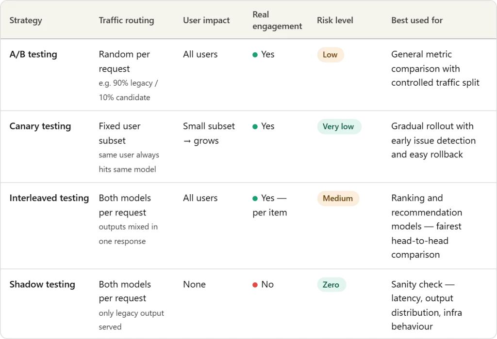
On this article, we discover 4 extensively used methods—A/B testing, Canary testing, Interleaved testing, and Shadow testing—that assist organizations safely deploy and validate new machine studying fashions in manufacturing environments.
A/B Testing
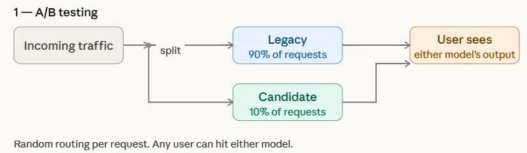
A/B testing is likely one of the most generally used methods for safely introducing a brand new machine studying mannequin in manufacturing. On this strategy, incoming visitors is break up between two variations of a system: the prevailing legacy mannequin (management) and the candidate mannequin (variation). The distribution is often non-uniform to restrict threat—for instance, 90% of requests might proceed to be served by the legacy mannequin, whereas solely 10% are routed to the candidate mannequin.
By exposing each fashions to real-world visitors, groups can examine downstream efficiency metrics comparable to click-through charge, conversions, engagement, or income. This managed experiment permits organizations to judge whether or not the candidate mannequin genuinely improves outcomes earlier than steadily rising its visitors share or absolutely changing the legacy mannequin.
Canary Testing
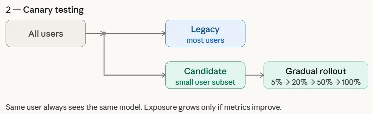
Canary testing is a managed rollout technique the place a brand new mannequin is first deployed to a small subset of customers earlier than being steadily launched to your complete consumer base. The title comes from an previous mining apply the place miners carried canary birds into coal mines to detect poisonous gases—the birds would react first, warning miners of hazard. Equally, in machine studying deployments, the candidate mannequin is initially uncovered to a restricted group of customers whereas the bulk proceed to be served by the legacy mannequin.
Not like A/B testing, which randomly splits visitors throughout all customers, canary testing targets a particular subset and progressively will increase publicity if efficiency metrics point out success. This gradual rollout helps groups detect points early and roll again rapidly if mandatory, lowering the chance of widespread influence.
Interleaved Testing
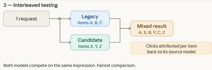
Interleaved testing evaluates a number of fashions by mixing their outputs throughout the similar response proven to customers. As an alternative of routing a whole request to both the legacy or candidate mannequin, the system combines predictions from each fashions in actual time. For instance, in a advice system, some gadgets within the advice checklist might come from the legacy mannequin, whereas others are generated by the candidate mannequin.
The system then logs downstream engagement indicators—comparable to click-through charge, watch time, or damaging suggestions—for every advice. As a result of each fashions are evaluated throughout the similar consumer interplay, interleaved testing permits groups to match efficiency extra straight and effectively whereas minimizing biases attributable to variations in consumer teams or visitors distribution.
Shadow Testing
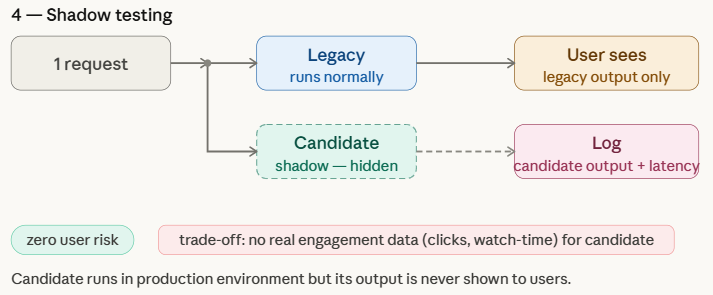
Shadow testing, often known as shadow deployment or darkish launch, permits groups to judge a brand new machine studying mannequin in an actual manufacturing setting with out affecting the consumer expertise. On this strategy, the candidate mannequin runs in parallel with the legacy mannequin and receives the identical reside requests because the manufacturing system. Nevertheless, solely the legacy mannequin’s predictions are returned to customers, whereas the candidate mannequin’s outputs are merely logged for evaluation.
This setup helps groups assess how the brand new mannequin behaves beneath real-world visitors and infrastructure circumstances, which are sometimes troublesome to duplicate in offline experiments. Shadow testing offers a low-risk approach to benchmark the candidate mannequin towards the legacy mannequin, though it can’t seize true consumer engagement metrics—comparable to clicks, watch time, or conversions—since its predictions are by no means proven to customers.
Simulating ML Mannequin Deployment Methods
Setting Up
Earlier than simulating any technique, we want two issues: a approach to symbolize incoming requests, and a stand-in for every mannequin.
Every mannequin is solely a perform that takes a request and returns a rating — a quantity that loosely represents how good that mannequin’s advice is. The legacy mannequin’s rating is capped at 0.35, whereas the candidate mannequin’s is capped at 0.55, making the candidate deliberately higher so we will confirm that every technique really detects the advance.
make_requests() generates 200 requests unfold throughout 40 customers, which supplies us sufficient visitors to see significant variations between methods whereas holding the simulation light-weight.
import random
import hashlib

random.seed(42)


def legacy_model(request):
    return {"mannequin": "legacy",    "rating": random.random() * 0.35}

def candidate_model(request):
    return {"mannequin": "candidate", "rating": random.random() * 0.55}

def make_requests(n=200):
    customers = [f"user_{i}" for i in range(40)]
    return [{"id": f"req_{i}", "user": random.choice(users)} for i in range(n)]

requests = make_requests()
A/B Testing
ab_route() is the core of this technique — for each incoming request, it attracts a random quantity and routes to the candidate mannequin provided that that quantity falls beneath 0.10, in any other case the request goes to legacy. This provides the candidate roughly 10% of visitors.
We then acquire the prediction scores from every mannequin individually and compute the typical on the finish. In an actual system, these scores would get replaced by precise engagement metrics like click-through charge or watch time — right here the rating simply stands in for “how good was this advice.”
print("── 1. A/B Testing ──────────────────────────────────────────")

CANDIDATE_TRAFFIC = 0.10   # 10 % of requests go to candidate

def ab_route(request):
    return candidate_model if random.random() < CANDIDATE_TRAFFIC else legacy_model

outcomes = {"legacy": [], "candidate": []}
for req in requests:
    mannequin  = ab_route(req)
    pred   = mannequin(req)
    outcomes[pred["model"]].append(pred["score"])

for title, scores in outcomes.gadgets():
    print(f"  {title:12s} | requests: {len(scores):3d} | avg rating: {sum(scores)/len(scores):.3f}")
Canary Testing
The important thing perform right here is get_canary_users(), which makes use of an MD5 hash to deterministically assign customers to the canary group. The necessary phrase is deterministic — sorting customers by their hash means the identical customers all the time find yourself within the canary group throughout runs, which mirrors how actual canary deployments work the place a particular consumer constantly sees the identical mannequin.
We then simulate three phases by merely increasing the fraction of canary customers — 5%, 20%, and 50%. For every request, routing is determined by whether or not the consumer belongs to the canary group, not by a random coin flip like in A/B testing. That is the basic distinction between the 2 methods: A/B testing splits by request, canary testing splits by consumer.
print("n── 2. Canary Testing ───────────────────────────────────────")

def get_canary_users(all_users, fraction):
    """Deterministic consumer task through hash -- steady throughout restarts."""
    n = max(1, int(len(all_users) * fraction))
    ranked = sorted(all_users, key=lambda u: hashlib.md5(u.encode()).hexdigest())
    return set(ranked[:n])

all_users = checklist(set(r["user"] for r in requests))

for part, fraction in [("Phase 1 (5%)", 0.05), ("Phase 2 (20%)", 0.20), ("Phase 3 (50%)", 0.50)]:
    canary_users = get_canary_users(all_users, fraction)
    scores = {"legacy": [], "candidate": []}
    for req in requests:
        mannequin = candidate_model if req["user"] in canary_users else legacy_model
        pred  = mannequin(req)
        scores[pred["model"]].append(pred["score"])
    print(f"  {part} | canary customers: {len(canary_users):second} "
          f"| legacy avg: {sum(scores['legacy'])/max(1,len(scores['legacy'])):.3f} "
          f"| candidate avg: {sum(scores['candidate'])/max(1,len(scores['candidate'])):.3f}")
Interleaved Testing
Each fashions run on each request, and interleave() merges their outputs by alternating gadgets — one from legacy, one from candidate, one from legacy, and so forth. Every merchandise is tagged with its supply mannequin, so when a consumer clicks one thing, we all know precisely which mannequin to credit score.
The small random.uniform(-0.05, 0.05) noise added to every merchandise’s rating simulates the pure variation you’d see in actual suggestions — two gadgets from the identical mannequin gained’t have similar high quality.
On the finish, we compute CTR individually for every mannequin’s gadgets. As a result of each fashions competed on the identical requests towards the identical customers on the similar time, there isn’t a confounding issue — any distinction in CTR is solely all the way down to mannequin high quality. That is what makes interleaved testing probably the most statistically clear comparability of the 4 methods.
print("n── 3. Interleaved Testing ──────────────────────────────────")

def interleave(pred_a, pred_b):
    """Alternate gadgets: A, B, A, B ... tagged with their supply mannequin."""
    items_a = [("legacy",    pred_a["score"] + random.uniform(-0.05, 0.05)) for _ in vary(3)]
    items_b = [("candidate", pred_b["score"] + random.uniform(-0.05, 0.05)) for _ in vary(3)]
    merged  = []
    for a, b in zip(items_a, items_b):
        merged += [a, b]
    return merged

clicks = {"legacy": 0, "candidate": 0}
proven  = {"legacy": 0, "candidate": 0}

for req in requests:
    pred_l = legacy_model(req)
    pred_c = candidate_model(req)
    for supply, rating in interleave(pred_l, pred_c):
        proven[source]  += 1
        clicks[source] += int(random.random() < rating)   # click on ~ rating

for title in ["legacy", "candidate"]:
    print(f"  {title:12s} | impressions: {proven[name]:4d} "
          f"| clicks: {clicks[name]:3d} "
          f"| CTR: {clicks[name]/proven[name]:.3f}")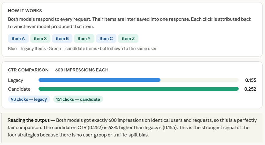
Shadow Testing
Each fashions run on each request, however the loop makes a transparent distinction — live_pred is what the consumer will get, shadow_pred goes straight into the log and nothing extra. The candidate’s output is rarely returned, by no means proven, by no means acted on. The log checklist is your complete level of shadow testing. In an actual system this is able to be written to a database or a knowledge warehouse, and engineers would later question it to match latency distributions, output patterns, or rating distributions towards the legacy mannequin — all with no single consumer being affected.
print("n── 4. Shadow Testing ───────────────────────────────────────")

log = []   # candidate's shadow log

for req in requests:
    # What the consumer sees
    live_pred   = legacy_model(req)

    # Shadow run -- by no means proven to consumer
    shadow_pred = candidate_model(req)

    log.append({
        "request_id":       req["id"],
        "legacy_score":     live_pred["score"],
        "candidate_score":  shadow_pred["score"],    # logged, not served
    })

avg_legacy    = sum(r["legacy_score"]    for r in log) / len(log)
avg_candidate = sum(r["candidate_score"] for r in log) / len(log)

print(f"  Legacy    avg rating (served):  {avg_legacy:.3f}")
print(f"  Candidate avg rating (logged):  {avg_candidate:.3f}")
print(f"  Observe: candidate rating has no click on validation -- shadow solely.")
Try the FULL Pocket book Right here. Additionally, be happy to observe us on Twitter and don’t neglect to affix our 120k+ ML SubReddit and Subscribe to our Publication. Wait! are you on telegram? now you possibly can be part of us on telegram as properly.

I’m a Civil Engineering Graduate (2022) from Jamia Millia Islamia, New Delhi, and I’ve a eager curiosity in Knowledge Science, particularly Neural Networks and their software in numerous areas.

