
The Mountain Trekker Analogy:
Think about you are a mountain trekker, standing someplace on the slopes of an enormous mountain vary. Your objective is to succeed in the bottom level within the valley, however there is a catch: you are blindfolded. With out the power to see all the panorama, how would you discover your option to the underside?
Instinctively, you would possibly really feel the bottom round you together with your toes, sensing which method is downhill. You’d then take a step in that route, the steepest descent. Repeating this course of, you’d progressively transfer nearer to the valley’s lowest level.
Within the realm of machine studying, this trekker’s journey mirrors the gradient descent algorithm. Here is how:
1) The Panorama: The mountainous terrain represents our value (or loss) operate,
J(θ). This operate measures the error or discrepancy between our mannequin’s predictions and the precise knowledge. Mathematically, it may very well be represented as:
the place
m is the variety of knowledge factors,hθ(x) is our mannequin’s prediction, and
y is the precise worth.
2) The Trekker’s Place: Your present place on the mountain corresponds to the present values of the mannequin’s parameters,θ. As you progress, these values change, altering the mannequin’s predictions.
3) Feeling the Floor: Simply as you sense the steepest descent together with your toes, in gradient descent, we compute the gradient,
∇J(θ). This gradient tells us the route of the steepest improve in our value operate. To minimise the price, we transfer in the other way. The gradient is given by:
The place:
m is the variety of coaching examples.
![]() is the prediction for the ith
is the prediction for the ith
coaching instance.
![]() is the jth function worth for the ith coaching instance.
is the jth function worth for the ith coaching instance.
![]() is the precise output for the ith
is the precise output for the ith
coaching instance.
4) Steps: The dimensions of the steps you are taking is analogous to the educational price in gradient descent, denoted by ?. A big step would possibly aid you descend quicker however dangers overshooting the valley’s backside. A smaller step is extra cautious however would possibly take longer to succeed in the minimal. The replace rule is:
5) Reaching the Backside: The iterative course of continues till you attain a degree the place you’re feeling no vital descent in any route. In gradient descent, that is when the change in the price operate turns into negligible, indicating that the algorithm has (hopefully) discovered the minimal.
In Conclusion
Gradient descent is a methodical and iterative course of, very like our blindfolded trekker looking for the valley’s lowest level. By combining instinct with mathematical rigor, we are able to higher perceive how machine studying fashions be taught, modify their parameters, and enhance their predictions.
Batch Gradient Descent computes the gradient utilizing all the dataset. This methodology gives a secure convergence and constant error gradient however will be computationally costly and gradual for big datasets.
SGD estimates the gradient utilizing a single, randomly chosen knowledge level. Whereas it may be quicker and is able to escaping native minima, it has a extra erratic convergence sample because of its inherent randomness, probably resulting in oscillations in the price operate.
Mini-Batch Gradient Descent strikes a steadiness between the 2 aforementioned strategies. It computes the gradient utilizing a subset (or “mini-batch”) of the dataset. This methodology accelerates convergence by benefiting from the computational benefits of matrix operations and presents a compromise between the soundness of Batch Gradient Descent and the pace of SGD.
Native Minima
Gradient descent can typically converge to a neighborhood minimal, which isn’t the optimum answer for all the operate. That is notably problematic in complicated landscapes with a number of valleys. To beat this, incorporating momentum helps the algorithm navigate via valleys with out getting caught. Moreover, superior optimization algorithms like Adam mix the advantages of momentum and adaptive studying charges to make sure extra sturdy convergence to world minima.
Vanishing & Exploding Gradients
In deep neural networks, as gradients are back-propagated, they’ll diminish to close zero (vanish) or develop exponentially (explode). Vanishing gradients decelerate coaching, making it exhausting for the community to be taught, whereas exploding gradients may cause the mannequin to diverge. To mitigate these points, gradient clipping units a threshold worth to stop gradients from changing into too giant. However, normalized initialization strategies, like He or Xavier initialization, be certain that the weights are set to optimum values initially, lowering the chance of those challenges.
import numpy as np

def gradient_descent(X, y, learning_rate=0.01, num_iterations=1000):
    m, n = X.form
    theta = np.zeros(n)  # Initialize weights/parameters
    cost_history = []  # To retailer values of the price operate over iterations

    for _ in vary(num_iterations):
        predictions = X.dot(theta)
        errors = predictions - y
        gradient = (1/m) * X.T.dot(errors)
        theta -= learning_rate * gradient

        # Compute and retailer the price for present iteration
        value = (1/(2*m)) * np.sum(errors**2)
        cost_history.append(value)

    return theta, cost_history

# Instance utilization:
# Assuming X is your function matrix with m samples and n options
# and y is your goal vector with m samples.
# Observe: You must add a bias time period (column of ones) to X if you need a bias time period in your mannequin.

# Pattern knowledge
X = np.array([[1, 1], [1, 2], [1, 3], [1, 4], [1, 5]])
y = np.array([2, 4, 5, 4, 5])

theta, cost_history = gradient_descent(X, y)

print("Optimum parameters:", theta)
print("Price historical past:", cost_history)
This code gives a primary gradient descent algorithm for linear regression. The operate gradient_descent takes within the function matrix X, goal vector y, a studying price, and the variety of iterations. It returns the optimized parameters (theta) and the historical past of the price operate over the iterations.
The left subplot reveals the price operate reducing over iterations.
The best subplot reveals the information factors and the road of greatest match obtained from gradient descent.
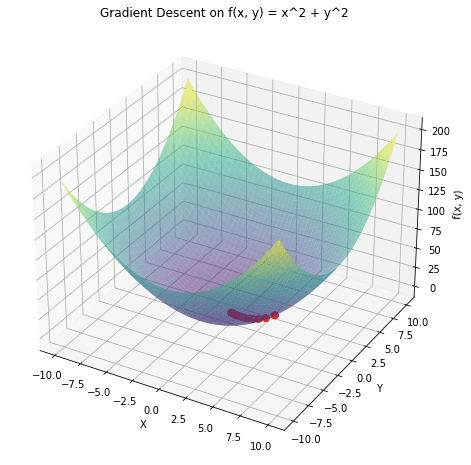
a 3D plot of the operate ![]() and overlay the trail taken by gradient descent in pink. The gradient descent begins from a random level and strikes in direction of the minimal of the operate.
and overlay the trail taken by gradient descent in pink. The gradient descent begins from a random level and strikes in direction of the minimal of the operate.
Inventory Value Prediction
Monetary analysts use gradient descent along with algorithms like linear regression to foretell future inventory costs based mostly on historic knowledge. By minimising the error between the expected and precise inventory costs, they’ll refine their fashions to make extra correct predictions.
Picture Recognition
Deep studying fashions, particularly Convolutional Neural Networks (CNNs), make use of gradient descent to optimise weights whereas coaching on huge datasets of pictures. For example, platforms like Fb use such fashions to routinely tag people in images by recognizing facial options. The optimization of those fashions ensures correct and environment friendly facial recognition.
Sentiment Evaluation
Corporations use gradient descent to coach fashions that analyse buyer suggestions, evaluations, or social media mentions to find out public sentiment about their services or products. By minimising the distinction between predicted and precise sentiments, these fashions can precisely classify suggestions as constructive, detrimental, or impartial, serving to companies gauge buyer satisfaction and tailor their methods accordingly.
Arun is a seasoned Senior Information Scientist with over 8 years of expertise in harnessing the ability of information to drive impactful enterprise options. He excels in leveraging superior analytics, predictive modelling, and machine studying to remodel complicated knowledge into actionable insights and strategic narratives. Holding a PGP in Machine Studying and Synthetic Intelligence from a famend establishment, Arun’s experience spans a broad spectrum of technical and strategic domains, making him a invaluable asset in any data-driven endeavour.

