Buyer Segmentation in Python: A Sensible Method

Picture by Writer | Created Utilizing Excalidraw and Flaticon

Buyer segmentation may also help companies tailor their advertising and marketing efforts and enhance buyer satisfaction. Right here’s how.

Functionally, buyer segmentation entails dividing a buyer base into distinct teams or segments—based mostly on shared traits and behaviors. By understanding the wants and preferences of every section, companies can ship extra personalised and efficient advertising and marketing campaigns, resulting in elevated buyer retention and income.

On this tutorial, we’ll discover buyer segmentation in Python by combining two elementary methods: RFM (Recency, Frequency, Financial) evaluation and Ok-Means clustering. RFM evaluation offers a structured framework for evaluating buyer habits, whereas Ok-means clustering presents a data-driven strategy to group prospects into significant segments. We’ll work with a real-world dataset from the retail business: the On-line Retail dataset from UCI machine studying repository.

From knowledge preprocessing to cluster evaluation and visualization, we’ll code our approach by every step. So let’s dive in!

Let’s begin by stating our purpose: By making use of RFM evaluation and Ok-means clustering to this dataset, we’d like to realize insights into buyer habits and preferences.

RFM Evaluation is an easy but highly effective methodology to quantify buyer habits. It evaluates prospects based mostly on three key dimensions:

• Recency (R): How just lately did a specific buyer make a purchase order?
• Frequency (F): How typically do they make purchases?
• Financial Worth (M): How a lot cash do they spend?

We’ll use the data within the dataset to compute the recency, frequency, and financial values. Then, we’ll map these values to the commonly used RFM rating scale of 1 – 5. 

In the event you’d like, you may discover and analyze additional utilizing these RFM scores. However we’ll attempt to establish buyer segments with comparable RFM traits. And for this, we’ll use Ok-Means clustering, an unsupervised machine studying algorithm that teams comparable knowledge factors into clusters.

So let’s begin coding!

🔗 Hyperlink to Google Colab pocket book.

Step 1 – Import Essential Libraries and Modules

First, let’s import the mandatory libraries and the precise modules as wanted:

import pandas as pd
import matplotlib.pyplot as plt
from sklearn.cluster import KMeans

We’d like pandas and matplotlib for knowledge exploration and visualization, and the KMeans class from scikit-learn’s cluster module to carry out Ok-Means clustering.

Step 2 – Load the Dataset

As talked about, we’ll use the On-line Retail dataset. The dataset accommodates buyer data: transactional data, together with buy dates, portions, costs, and buyer IDs. 

Let’s learn within the knowledge that’s initially in an excel file from its URL right into a pandas dataframe.

# Load the dataset from UCI repository
url = "https://archive.ics.uci.edu/ml/machine-learning-databases/00352/Onlinepercent20Retail.xlsx"
knowledge = pd.read_excel(url)

Alternatively, you may obtain the dataset and browse the excel file right into a pandas dataframe.

Step 3 – Discover and Clear the Dataset

Now let’s begin exploring the dataset. Have a look at the primary few rows of the dataset:

Output of information.head()

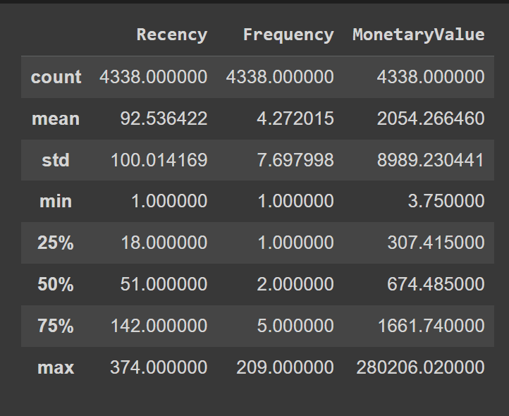
Now name the describe() methodology on the dataframe to know the numerical options higher:

We see that the “CustomerID” column is at present a floating level worth. Once we clear the info, we’ll solid it into an integer:
 

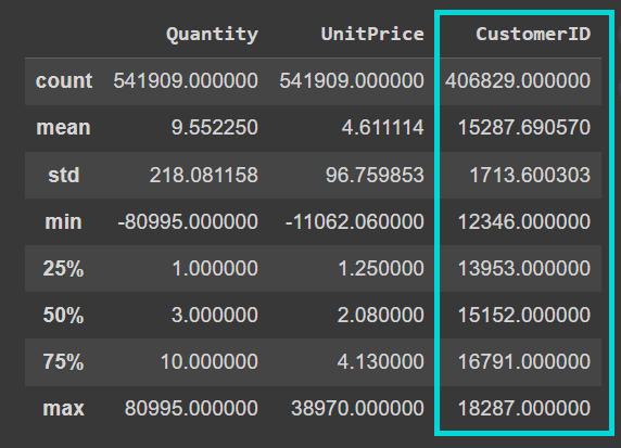
Output of information.describe()

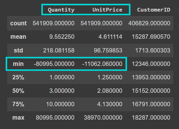
Additionally observe that the dataset is kind of noisy. The “Amount” and “UnitPrice” columns comprise detrimental values:

Output of information.describe()

Let’s take a better take a look at the columns and their knowledge varieties:

We see that the dataset has over 541K data and the “Description” and “CustomerID” columns comprise lacking values:
 

# Verify for lacking values in every column
missing_values = knowledge.isnull().sum()
print(missing_values)

As anticipated, the “CustomerID” and “Description” columns comprise lacking values: 

For our evaluation, we don’t want the product description contained within the “Description” column. Nonetheless, we’d like the “CustomerID” for the subsequent steps in our evaluation. So let’s drop the data with lacking “CustomerID”:

# Drop rows with lacking CustomerID
knowledge.dropna(subset=['CustomerID'], inplace=True)

Additionally recall that the values “Amount” and “UnitPrice” columns needs to be strictly non-negative. However they comprise detrimental values. So let’s additionally drop the data with detrimental values for  “Amount” and “UnitPrice”:

# Take away rows with detrimental Amount and Worth
knowledge = knowledge[(data['Quantity'] > 0) & (knowledge['UnitPrice'] > 0)]

Let’s additionally convert the “CustomerID” to an integer:

knowledge['CustomerID'] = knowledge['CustomerID'].astype(int)

# Confirm the info kind conversion
print(knowledge.dtypes)

Step 4 – Compute Recency, Frequency, and Financial Worth

Let’s begin out by defining a reference date snapshot_date that’s a day later than the newest date within the “InvoiceDate” column:

snapshot_date = max(knowledge['InvoiceDate']) + pd.DateOffset(days=1)

Subsequent, create a “Complete” column that accommodates Amount*UnitPrice for all of the data:

knowledge['Total'] = knowledge['Quantity'] * knowledge['UnitPrice']

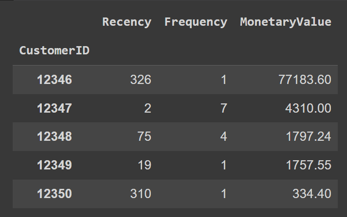
To calculate the Recency, Frequency, and MonetaryValue, we calculate the next—grouped by CustomerID:

• For recency, we’ll calculate the distinction between the newest buy date and a reference date (snapshot_date). This provides the variety of days because the buyer’s final buy. So smaller values point out {that a} buyer has made a purchase order extra just lately. However once we speak about recency scores, we’d need prospects who purchased just lately to have a better recency rating, sure? We’ll deal with this within the subsequent step.
• As a result of frequency measures how typically a buyer makes purchases, we’ll calculate it as the overall variety of distinctive invoices or transactions made by every buyer.
• Financial worth quantifies how a lot cash a buyer spends. So we’ll discover the typical of the overall financial worth throughout transactions.

rfm = knowledge.groupby('CustomerID').agg({
    'InvoiceDate': lambda x: (snapshot_date - x.max()).days,
    'InvoiceNo': 'nunique',
    'Complete': 'sum'
})

Let’s rename the columns for readability:

rfm.rename(columns={'InvoiceDate': 'Recency', 'InvoiceNo': 'Frequency', 'Complete': 'MonetaryValue'}, inplace=True)
rfm.head()

Step 5 – Map RFM Values onto a 1-5 Scale 

Now let’s map the “Recency”, “Frequency”, and “MonetaryValue” columns to tackle values in a scale of 1-5; one in all {1,2,3,4,5}.

We’ll primarily assign the values to 5 completely different bins, and map every bin to a price. To assist us repair the bin edges, let’s use the quantile values of the “Recency”, “Frequency”, and “MonetaryValue” columns:

Right here’s how we outline the customized bin edges:

# Calculate customized bin edges for Recency, Frequency, and Financial scores
recency_bins = [rfm['Recency'].min()-1, 20, 50, 150, 250, rfm['Recency'].max()]
frequency_bins = [rfm['Frequency'].min() - 1, 2, 3, 10, 100, rfm['Frequency'].max()]
monetary_bins = [rfm['MonetaryValue'].min() - 3, 300, 600, 2000, 5000, rfm['MonetaryValue'].max()]

Now that we’ve outlined the bin edges, let’s map the scores to corresponding labels between 1 and 5 (each inclusive):

# Calculate Recency rating based mostly on customized bins 
rfm['R_Score'] = pd.minimize(rfm['Recency'], bins=recency_bins, labels=vary(1, 6), include_lowest=True)

# Reverse the Recency scores in order that increased values point out more moderen purchases
rfm['R_Score'] = 5 - rfm['R_Score'].astype(int) + 1

# Calculate Frequency and Financial scores based mostly on customized bins
rfm['F_Score'] = pd.minimize(rfm['Frequency'], bins=frequency_bins, labels=vary(1, 6), include_lowest=True).astype(int)
rfm['M_Score'] = pd.minimize(rfm['MonetaryValue'], bins=monetary_bins, labels=vary(1, 6), include_lowest=True).astype(int)

Discover that the R_Score, based mostly on the bins, is 1 for current purchases 5 for all purchases remodeled 250 days in the past. However we’d like the newest purchases to have an R_Score of 5 and purchases remodeled 250 days in the past to have an R_Score of 1.

To attain the specified mapping, we do: 5 - rfm['R_Score'].astype(int) + 1.

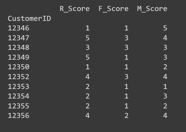
Let’s take a look at the primary few rows of the R_Score, F_Score, and M_Score columns:

# Print the primary few rows of the RFM DataFrame to confirm the scores
print(rfm[['R_Score', 'F_Score', 'M_Score']].head(10))

In the event you’d like, you need to use these R, F, and M scores to hold out an in-depth evaluation. Or use clustering to establish segments with comparable RFM traits. We’ll select the latter!

Step 6 – Carry out Ok-Means Clustering

Ok-Means clustering is delicate to the size of options. As a result of the R, F, and M values are all on the identical scale, we are able to proceed to carry out clustering with out additional scaling the options. 

Let’s extract the R, F, and M scores to carry out Ok-Means clustering:

# Extract RFM scores for Ok-means clustering
X = rfm[['R_Score', 'F_Score', 'M_Score']]

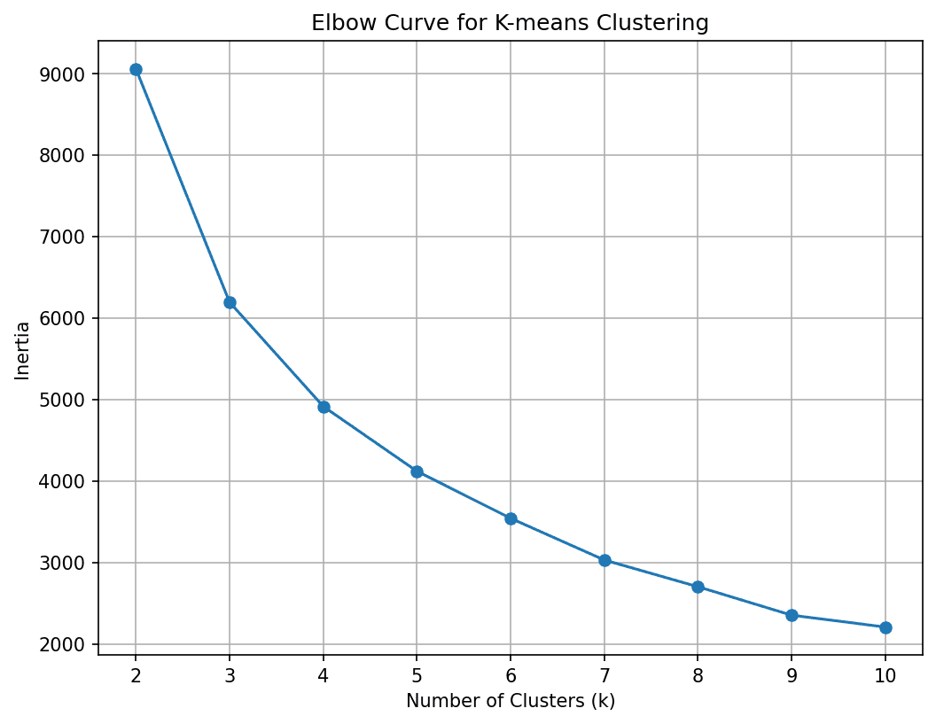
Subsequent, we have to discover the optimum variety of clusters. For this let’s run the Ok-Means algorithm for a variety of Ok values and use the elbow methodology to select the optimum Ok:

# Calculate inertia (sum of squared distances) for various values of ok
inertia = []
for ok in vary(2, 11):
    kmeans = KMeans(n_clusters=ok, n_init= 10, random_state=42)
    kmeans.match(X)
    inertia.append(kmeans.inertia_)

# Plot the elbow curve
plt.determine(figsize=(8, 6),dpi=150)
plt.plot(vary(2, 11), inertia, marker="o")
plt.xlabel('Variety of Clusters (ok)')
plt.ylabel('Inertia')
plt.title('Elbow Curve for Ok-means Clustering')
plt.grid(True)
plt.present()

We see that the curve elbows out at 4 clusters. So let’s divide the shopper base into 4 segments.

We’ve fastened Ok to 4. So let’s run the Ok-Means algorithm to get the cluster assignments for all factors within the dataset:

# Carry out Ok-means clustering with greatest Ok
best_kmeans = KMeans(n_clusters=4, n_init=10, random_state=42)
rfm['Cluster'] = best_kmeans.fit_predict(X)

Step 7 – Interpret the Clusters to Determine Buyer Segments 

Now that we’ve got the clusters, let’s attempt to characterize them based mostly on the RFM scores.

# Group by cluster and calculate imply values
cluster_summary = rfm.groupby('Cluster').agg({
    'R_Score': 'imply',
    'F_Score': 'imply',
    'M_Score': 'imply'
}).reset_index()

The typical R, F, and M scores for every cluster ought to already provide you with an thought of the traits. 

However let’s visualize the typical R, F, and M scores for the clusters so it’s straightforward to interpret:

colours = ['#3498db', '#2ecc71', '#f39c12','#C9B1BD']

# Plot the typical RFM scores for every cluster
plt.determine(figsize=(10, 8),dpi=150)

# Plot Avg Recency
plt.subplot(3, 1, 1)
bars = plt.bar(cluster_summary.index, cluster_summary['R_Score'], shade=colours)
plt.xlabel('Cluster')
plt.ylabel('Avg Recency')
plt.title('Common Recency for Every Cluster')

plt.grid(True, linestyle="--", alpha=0.5)
plt.legend(bars, cluster_summary.index, title="Clusters")

# Plot Avg Frequency
plt.subplot(3, 1, 2)
bars = plt.bar(cluster_summary.index, cluster_summary['F_Score'], shade=colours)
plt.xlabel('Cluster')
plt.ylabel('Avg Frequency')
plt.title('Common Frequency for Every Cluster')
plt.grid(True, linestyle="--", alpha=0.5)
plt.legend(bars, cluster_summary.index, title="Clusters")

# Plot Avg Financial
plt.subplot(3, 1, 3)
bars = plt.bar(cluster_summary.index, cluster_summary['M_Score'], shade=colours)
plt.xlabel('Cluster')
plt.ylabel('Avg Financial')
plt.title('Common Financial Worth for Every Cluster')
plt.grid(True, linestyle="--", alpha=0.5)
plt.legend(bars, cluster_summary.index, title="Clusters")

plt.tight_layout()
plt.present()

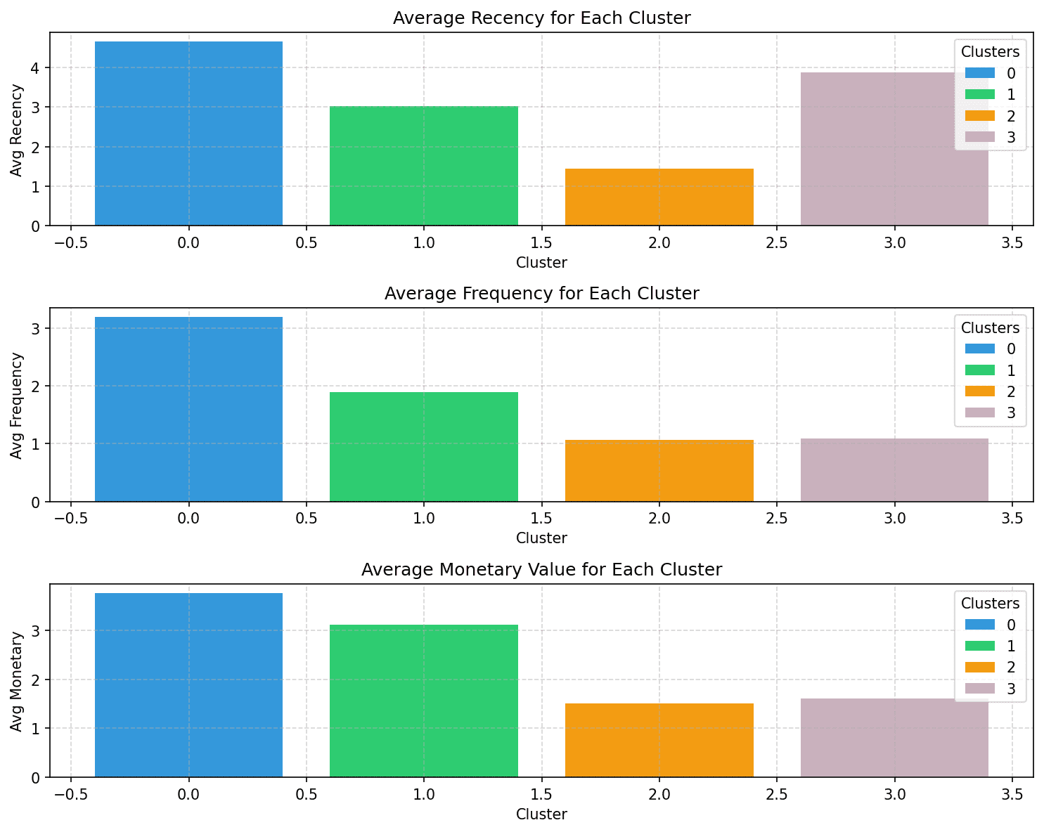
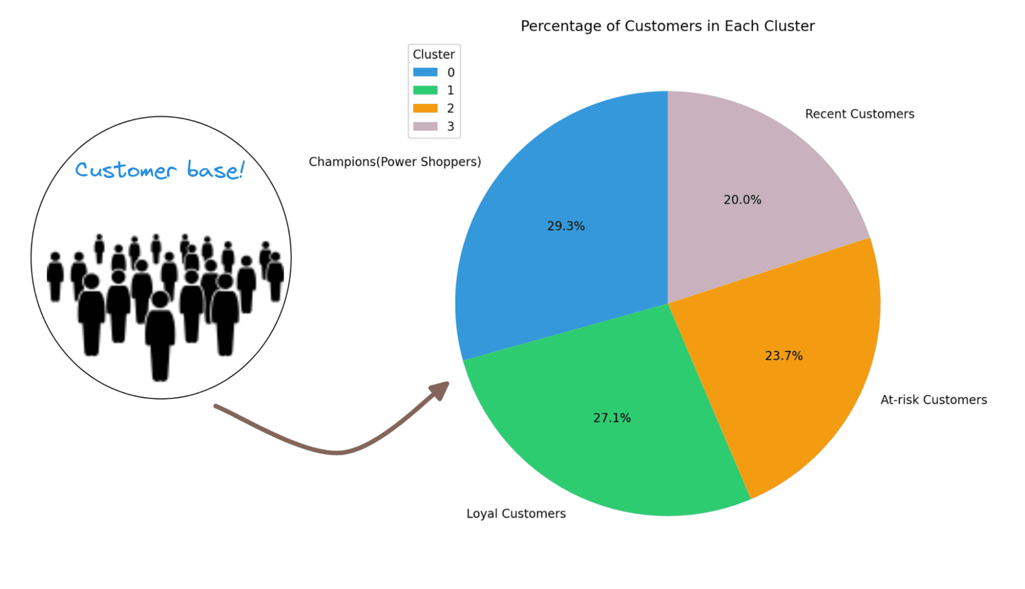
Discover how the shoppers in every of the segments might be characterised based mostly on the recency, frequency, and financial values:

• Cluster 0: Of all of the 4 clusters, this cluster has the highest recency, frequency, and financial values. Let’s name the shoppers on this cluster champions (or energy consumers).
• Cluster 1: This cluster is characterised by average recency, frequency, and financial values. These prospects nonetheless spend extra and buy extra often than clusters 2 and three. Let’s name them loyal prospects.
• Cluster 2: Clients on this cluster are inclined to spend much less. They don’t purchase typically, and haven’t made a purchase order just lately both. These are seemingly inactive or at-risk prospects.
• Cluster 3: This cluster is characterised by excessive recency and comparatively decrease frequency and average financial values. So these are current prospects who can doubtlessly turn into long-term prospects.

Listed here are some examples of how one can tailor advertising and marketing efforts—to focus on prospects in every section—to reinforce buyer engagement and retention:

• For Champions/Energy Buyers: Provide personalised particular reductions, early entry, and different premium perks to make them really feel valued and appreciated.
• For Loyal Clients: Appreciation campaigns, referral bonuses, and rewards for loyalty.
• For At-Threat Clients: Re-engagement efforts that embrace working reductions or promotions to encourage shopping for.
• For Latest Clients: Focused campaigns educating them concerning the model and reductions on subsequent purchases. 

It’s additionally useful to know what share of shoppers are within the completely different segments. This can additional assist streamline advertising and marketing efforts and develop your small business.

Let’s visualize the distribution of the completely different clusters utilizing a pie chart:

cluster_counts = rfm['Cluster'].value_counts()

colours = ['#3498db', '#2ecc71', '#f39c12','#C9B1BD']
# Calculate the overall variety of prospects
total_customers = cluster_counts.sum()

# Calculate the proportion of shoppers in every cluster
percentage_customers = (cluster_counts / total_customers) * 100

labels = ['Champions(Power Shoppers)','Loyal Customers','At-risk Customers','Recent Customers']

# Create a pie chart
plt.determine(figsize=(8, 8),dpi=200)
plt.pie(percentage_customers, labels=labels, autopct="%1.1f%%", startangle=90, colours=colours)
plt.title('Proportion of Clients in Every Cluster')
plt.legend(cluster_summary['Cluster'], title="Cluster", loc="higher left")

plt.present()

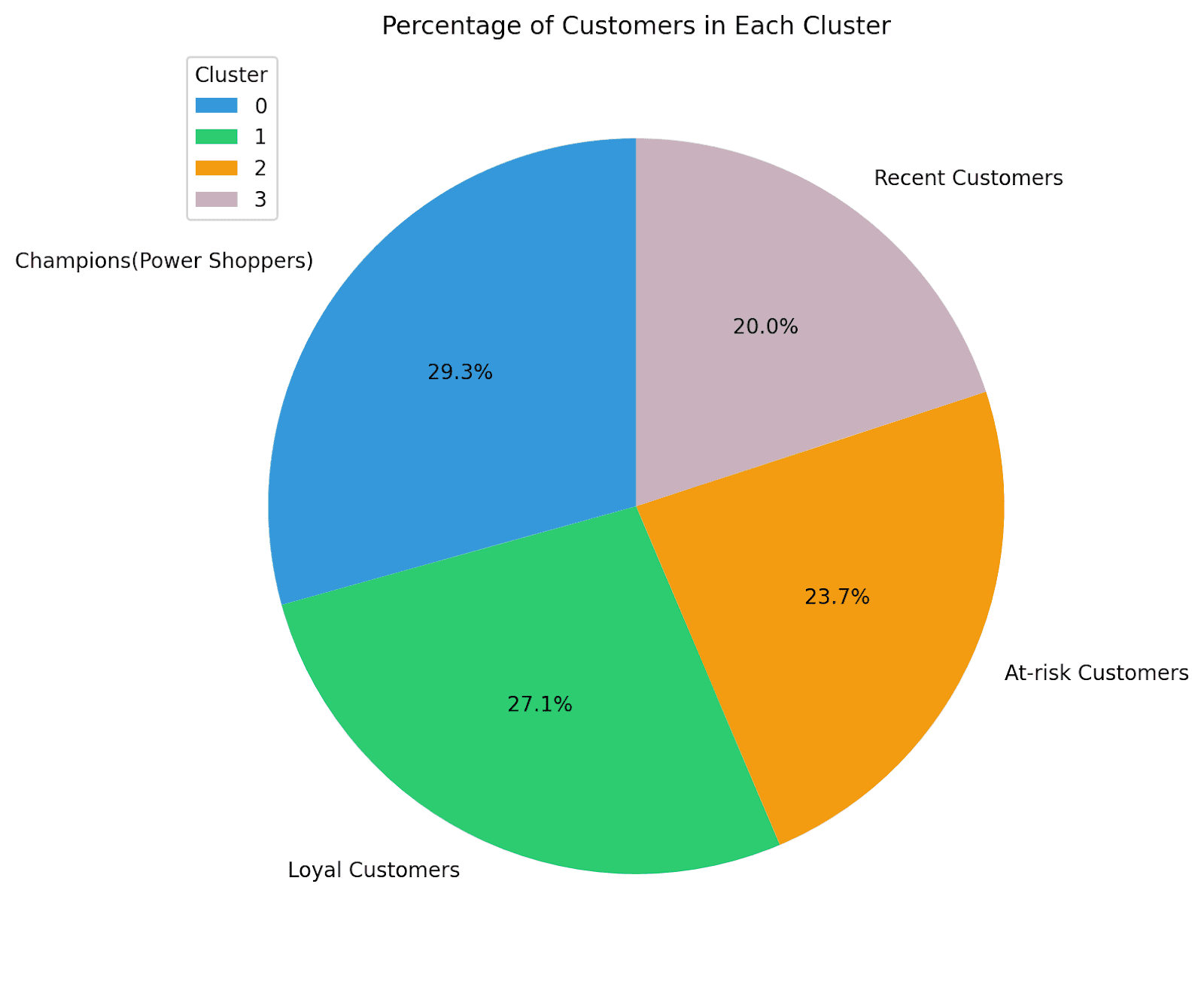
Right here we go! For this instance, we’ve got fairly an excellent distribution of shoppers throughout segments. So we are able to make investments effort and time in retaining current prospects, re-engaging with at-risk prospects, and educating current prospects.

And that’s a wrap! We went from over 154K buyer data to 4 clusters in 7 straightforward steps. I hope you perceive how buyer segmentation means that you can make data-driven selections that affect enterprise development and buyer satisfaction by permitting for:

• Personalization: Segmentation permits companies to tailor their advertising and marketing messages, product suggestions, and promotions to every buyer group’s particular wants and pursuits.
• Improved Concentrating on: By figuring out high-value and at-risk prospects, companies can allocate assets extra effectively, focusing efforts the place they’re most certainly to yield outcomes.
• Buyer Retention: Segmentation helps companies create retention methods by understanding what retains prospects engaged and glad.

As a subsequent step, attempt making use of this strategy to a different dataset, doc your journey, and share with the neighborhood! However keep in mind, efficient buyer segmentation and working focused campaigns requires a great understanding of your buyer base—and the way the shopper base evolves. So it requires periodic evaluation to refine your methods over time.

The On-line Retail Dataset is licensed beneath a Inventive Commons Attribution 4.0 Worldwide (CC BY 4.0) license:

On-line Retail. (2015). UCI Machine Studying Repository. https://doi.org/10.24432/C5BW33.
 
 
Bala Priya C is a developer and technical author from India. She likes working on the intersection of math, programming, knowledge science, and content material creation. Her areas of curiosity and experience embrace DevOps, knowledge science, and pure language processing. She enjoys studying, writing, coding, and occasional! At the moment, she’s engaged on studying and sharing her data with the developer neighborhood by authoring tutorials, how-to guides, opinion items, and extra.
 

Bala Priya C is a developer and technical author from India. She likes working on the intersection of math, programming, knowledge science, and content material creation. Her areas of curiosity and experience embrace DevOps, knowledge science, and pure language processing. She enjoys studying, writing, coding, and occasional! At the moment, she’s engaged on studying and sharing her data with the developer neighborhood by authoring tutorials, how-to guides, opinion items, and extra.