Sample Page Title

Picture by Creator

Knowledge cleansing is a important a part of any information evaluation course of. It is the step the place you take away errors, deal with lacking information, and make it possible for your information is in a format that you could work with. And not using a well-cleaned dataset, any subsequent analyses could be skewed or incorrect.

This text introduces you to a number of key methods for information cleansing in Python, utilizing highly effective libraries like pandas, numpy, seaborn, and matplotlib.

Earlier than diving into the mechanics of knowledge cleansing, let’s perceive its significance. Actual-world information is commonly messy. It might probably include duplicate entries, incorrect or inconsistent information varieties, lacking values, irrelevant options, and outliers. All these components can result in deceptive conclusions when analyzing information. This makes information cleansing an indispensable a part of the information science lifecycle.

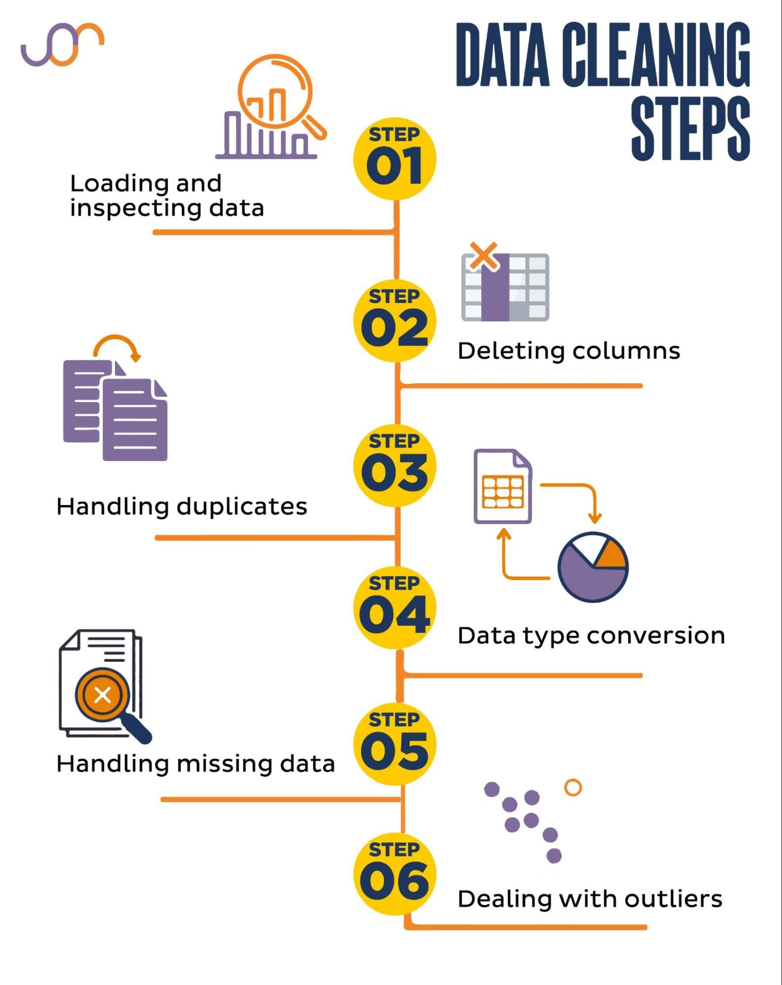
We’ll cowl the next information cleansing duties.
 

Picture by Creator

Earlier than getting began, let’s import the mandatory libraries. We’ll be utilizing pandas for information manipulation, and seaborn and matplotlib for visualizations.

We’ll additionally import the datetime Python module for manipulating the dates.

import pandas as pd
import seaborn as sns
import datetime as dt
import matplotlib.pyplot as plt
import matplotlib.ticker as ticker

First, we’ll must load our information. On this instance, we’ll load a CSV file utilizing pandas. We additionally add the delimiter argument.

df = pd.read_csv('F:KDNuggetsKDN Mastering the Artwork of Knowledge Cleansing in Pythonproperty.csv', delimiter=";")

Subsequent, it is vital to examine the information to know its construction, what sort of variables we’re working with, and whether or not there are any lacking values. Because the information we imported isn’t big, let’s take a look on the complete dataset.

# Take a look at all of the rows of the dataframe
show(df)

Right here’s how the dataset seems to be.

You possibly can instantly see there are some lacking values. Additionally, the date codecs are inconsistent.

Now, let’s check out the DataFrame abstract utilizing the information() technique.

# Get a concise abstract of the dataframe
print(df.data())

Right here’s the code output.

We are able to see that solely the column square_feet doesn’t have any NULL values, so we’ll in some way must deal with this. Additionally, the columns advertisement_date, and sale_date are the thing information kind, although this ought to be a date.

The column location is totally empty. Do we’d like it?

We’ll present you find out how to deal with these points. We’ll begin by studying find out how to delete pointless columns.

There are two columns within the dataset that we don’t want in our information evaluation, so we’ll take away them.

The primary column is purchaser. We don’t want it, as the client’s identify doesn’t influence the evaluation.

We’re utilizing the drop() technique with the required column identify. We set the axis to 1 to specify that we need to delete a column. Additionally, the inplace argument is about to True in order that we modify the prevailing DataFrame, and never create a brand new DataFrame with out the eliminated column.

df.drop('purchaser', axis = 1, inplace = True)

The second column we need to take away is location. Whereas it could be helpful to have this data, it is a fully empty column, so let’s simply take away it.

We take the identical method as with the primary column.

df.drop('location', axis = 1, inplace = True)

After all, you may take away these two columns concurrently.

df = df.drop(['buyer', 'location'], axis=1)

Each approaches return the next dataframe.

Duplicate information can happen in your dataset for varied causes and may skew your evaluation.

Let’s detect the duplicates in our dataset. Right here’s find out how to do it.

The under code makes use of the strategy duplicated() to contemplate duplicates in the entire dataset. Its default setting is to contemplate the primary incidence of a worth as distinctive and the next occurrences as duplicates. You possibly can modify this habits utilizing the maintain parameter. For example, df.duplicated(maintain=False) would mark all duplicates as True, together with the primary incidence.

# Detecting duplicates
duplicates = df[df.duplicated()]
duplicates

Right here’s the output.

The row with index 3 has been marked as duplicate as a result of row 2 with the identical values is its first incidence.

Now we have to take away duplicates, which we do with the next code.

# Detecting duplicates
duplicates = df[df.duplicated()]
duplicates

The drop_duplicates() perform considers all columns whereas figuring out duplicates. If you wish to take into account solely sure columns, you may go them as an inventory to this perform like this: df.drop_duplicates(subset=[‘column1’, ‘column2’]).

As you may see, the duplicate row has been dropped. Nonetheless, the indexing stayed the identical, with index 3 lacking. We’ll tidy this up by resetting indices.

df = df.reset_index(drop=True)

This activity is carried out by utilizing the reset_index() perform.  The drop=True argument is used to discard the unique index. If you don’t embrace this argument, the outdated index might be added as a brand new column in your DataFrame. By setting drop=True, you’re telling pandas to overlook the outdated index and reset it to the default integer index.

For apply, attempt to take away duplicates from this Microsoft dataset.

Generally, information varieties could be incorrectly set. For instance, a date column could be interpreted as strings. It is advisable convert these to their acceptable varieties.

In our dataset, we’ll try this for the columns advertisement_date and sale_date, as they’re proven as the thing information kind. Additionally, the date dates are formatted otherwise throughout the rows. We have to make it constant, together with changing it so far.

The best manner is to make use of the to_datetime() technique. Once more, you are able to do that column by column, as proven under.

When doing that, we set the dayfirst argument to True as a result of some dates begin with the day first.

# Changing advertisement_date column to datetime
df['advertisement_date'] = pd.to_datetime(df['advertisement_date'], dayfirst = True)

# Changing sale_date column to datetime
df['sale_date'] = pd.to_datetime(df['sale_date'], dayfirst = True)

You too can convert each columns on the similar time by utilizing the apply() technique with to_datetime().

# Changing advertisement_date and sale_date columns to datetime
df[['advertisement_date', 'sale_date']] = df[['advertisement_date', 'sale_date']].apply(pd.to_datetime, dayfirst =  True)

Each approaches provide the similar consequence.

Now the dates are in a constant format. We see that not all information has been transformed. There’s one NaT worth in advertisement_date and two in sale_date. This implies the date is lacking.

Let’s test if the columns are transformed to dates by utilizing the data() technique.

# Get a concise abstract of the dataframe
print(df.data())

As you may see, each columns should not in datetime64[ns] format.

Now, attempt to convert the information from TEXT to NUMERIC on this Airbnb dataset.

Actual-world datasets typically have lacking values. Dealing with lacking information is significant, as sure algorithms can’t deal with such values.

Our instance additionally has some lacking values, so let’s check out the 2 most standard approaches to dealing with lacking information.

Deleting Rows With Lacking Values

If the variety of rows with lacking information is insignificant in comparison with the whole variety of observations, you may take into account deleting these rows.

In our instance, the final row has no values besides the sq. ft and commercial date. We are able to’t use such information, so let’s take away this row.

Right here’s the code the place we point out the row’s index.

The DataFrame now seems to be like this.

The final row has been deleted, and our DataFrame now seems to be higher. Nonetheless, there are nonetheless some lacking information which we’ll deal with utilizing one other method.

Imputing Lacking Values

If in case you have important lacking information, a greater technique than deleting may very well be imputation. This course of includes filling in lacking values primarily based on different information. For numerical information, widespread imputation strategies contain utilizing a measure of central tendency (imply, median, mode).

In our already modified DataFrame, we’ve NaT (Not a Time) values within the columns advertisement_date and sale_date. We’ll impute these lacking values utilizing the imply() technique.

The code makes use of the fillna() technique to search out and fill the null values with the imply worth.

# Imputing values for numerical columns
df['advertisement_date'] = df['advertisement_date'].fillna(df['advertisement_date'].imply())
df['sale_date'] = df['sale_date'].fillna(df['sale_date'].imply())

You too can do the identical factor in a single line of code. We use the apply() to use the perform outlined utilizing lambda. Similar as above, this perform makes use of the fillna() and imply() strategies to fill within the lacking values.

# Imputing values for a number of numerical columns
df[['advertisement_date', 'sale_date']] = df[['advertisement_date', 'sale_date']].apply(lambda x: x.fillna(x.imply()))

The output in each instances seems to be like this.

Our sale_date column now has occasions which we don’t want. Let’s take away them.

We’ll use the strftime() technique, which converts the dates to their string illustration and a selected format.

df['sale_date'] = df['sale_date'].dt.strftime('%Y-%m-%d')

The dates now look all tidy.

If it’s essential to use strftime() on a number of columns, you may once more use lambda the next manner.

df[['date1_formatted', 'date2_formatted']] = df[['date1', 'date2']].apply(lambda x: x.dt.strftime('%Y-%m-%d'))

Now, let’s see how we are able to impute lacking categorical values.

Categorical information is a kind of knowledge that’s used to group data with comparable traits. Every of those teams is a class. Categorical information can tackle numerical values (similar to “1” indicating “male” and “2” indicating “feminine”), however these numbers should not have mathematical that means. You possibly can’t add them collectively, as an illustration.

Categorical information is usually divided into two classes:

1. Nominal information: That is when the classes are solely labeled and can’t be organized in any explicit order. Examples embrace gender (male, feminine), blood kind (A, B, AB, O), or shade (purple, inexperienced, blue).

1. Ordinal information: That is when the classes could be ordered or ranked. Whereas the intervals between the classes should not equally spaced, the order of the classes has a that means. Examples embrace ranking scales (1 to five ranking of a film), an training degree (highschool, undergraduate, graduate), or levels of most cancers (Stage I, Stage II, Stage III).

For imputing lacking categorical information, the mode is usually used. In our instance, the column property_category is categorical (nominal) information, and there’s information lacking in two rows.

Let’s change the lacking values with mode.

# For categorical columns
df['property_category'] = df['property_category'].fillna(df['property_category'].mode()[0])

This code makes use of the fillna() perform to exchange all of the NaN values within the property_category column. It replaces it with mode.

Moreover, the [0] half is used to extract the primary worth from this Collection. If there are a number of modes, this may choose the primary one. If there’s just one mode, it nonetheless works positive.

Right here’s the output.

The information now seems to be fairly good. The one factor that’s remaining is to see if there are outliers.

You possibly can apply coping with nulls on this Meta interview query, the place you’ll have to exchange NULLs with zeros.

Outliers are information factors in a dataset which are distinctly totally different from the opposite observations. They might lie exceptionally removed from the opposite values within the information set, residing exterior an general sample. They’re thought of uncommon because of their values both being considerably larger or decrease in comparison with the remainder of the information.

Outliers can come up because of varied causes similar to:

• Measurement or enter errors
• Knowledge corruption
• True statistical anomalies

Outliers can considerably influence the outcomes of your information evaluation and statistical modeling. They’ll result in a skewed distribution, bias, or invalidate the underlying statistical assumptions, distort the estimated mannequin match, scale back the predictive accuracy of predictive fashions, and result in incorrect conclusions.

Some generally used strategies to detect outliers are Z-score, IQR (Interquartile Vary), field plots, scatter plots, and information visualization methods. In some superior instances, machine studying strategies are used as effectively.

Visualizing information may also help determine outliers. Seaborn’s boxplot is useful for this.

plt.determine(figsize=(10, 6))
sns.boxplot(information=df[['advertised_price', 'sale_price']])

We use the plt.determine() to set the width and top of the determine in inches.

Then we create the boxplot for the columns advertised_price and sale_price, which seems to be like this.

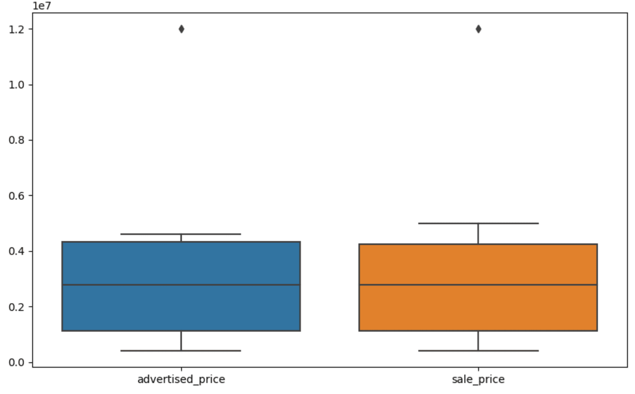
The plot could be improved for simpler use by including this to the above code.

plt.xlabel('Costs')
plt.ylabel('USD')
plt.ticklabel_format(model="plain", axis="y")
formatter = ticker.FuncFormatter(lambda x, p: format(x, ',.2f'))
plt.gca().yaxis.set_major_formatter(formatter)

We use the above code to set the labels for each axes. We additionally discover that the values on the y-axis are within the scientific notation, and we are able to’t use that for the value values. So we modify this to plain model utilizing the plt.ticklabel_format() perform.

Then we create the formatter that can present the values on the y-axis with commas as thousand separators and decimal dots. The final code line applies this to the axis.

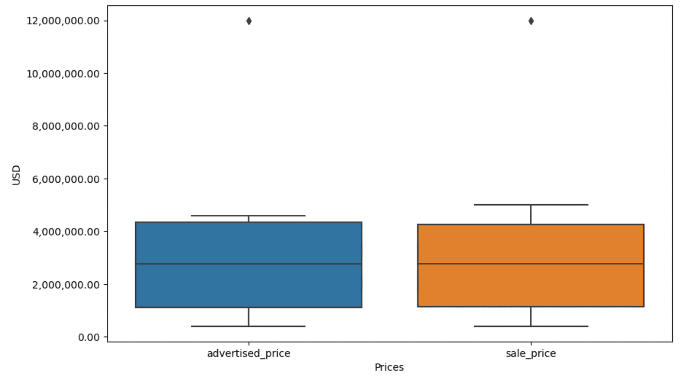
The output now seems to be like this.

Now, how can we determine and take away the outlier?

One of many methods is to make use of the IQR technique.

IQR, or Interquartile Vary, is a statistical technique used to measure variability by dividing an information set into quartiles. Quartiles divide a rank-ordered information set into 4 equal components, and values inside the vary of the primary quartile (twenty fifth percentile) and the third quartile (seventy fifth percentile) make up the interquartile vary.

The interquartile vary is used to determine outliers within the information. Here is the way it works:

1. First, calculate the primary quartile (Q1), the third quartile (Q3), after which decide the IQR. The IQR is computed as Q3 – Q1.
2. Any worth under Q1 – 1.5IQR or above Q3 + 1.5IQR is taken into account an outlier.

On our boxplot, the field truly represents the IQR. The road contained in the field is the median (or second quartile). The ‘whiskers’ of the boxplot characterize the vary inside 1.5*IQR from Q1 and Q3.

Any information factors exterior these whiskers could be thought of outliers. In our case, it’s the worth of $12,000,000. For those who take a look at the boxplot, you’ll see how clearly that is represented, which exhibits why information visualization is vital in detecting outliers.

Now, let’s take away the outliers by utilizing the IQR technique in Python code. First, we’ll take away the marketed worth outliers.

Q1 = df['advertised_price'].quantile(0.25)
Q3 = df['advertised_price'].quantile(0.75)
IQR = Q3 - Q1
df = df[~((df['advertised_price'] < (Q1 - 1.5 * IQR)) |(df['advertised_price'] > (Q3 + 1.5 * IQR)))]

We first calculate the primary quartile (or the twenty fifth percentile) utilizing the quantile() perform. We do the identical for the third quartile or the seventy fifth percentile.

They present the values under which 25% and 75% of the information fall, respectively.

Then we calculate the distinction between the quartiles. The whole lot to this point is simply translating the IQR steps into Python code.

As a remaining step, we take away the outliers. In different phrases, all information lower than Q1 – 1.5 * IQR or greater than Q3 + 1.5 * IQR.

The ‘~’ operator negates the situation, so we’re left with solely the information that aren’t outliers.

Then we are able to do the identical with the sale worth.

Q1 = df['sale_price'].quantile(0.25)
Q3 = df['sale_price'].quantile(0.75)
IQR = Q3 - Q1
df = df[~((df['sale_price'] < (Q1 - 1.5 * IQR)) |(df['sale_price'] > (Q3 + 1.5 * IQR)))]

After all, you are able to do it in a extra succinct manner utilizing the for loop.

for column in ['advertised_price', 'sale_price']:
    Q1 = df[column].quantile(0.25)
    Q3 = df[column].quantile(0.75)
    IQR = Q3 - Q1
    df = df[~((df[column] < (Q1 - 1.5 * IQR)) |(df[column] > (Q3 + 1.5 * IQR)))]

The loop iterates of the 2 columns. For every column, it calculates the IQR after which removes the rows within the DataFrame.

Please notice that this operation is completed sequentially, first for advertised_price after which for sale_price. Consequently, the DataFrame is modified in-place for every column, and rows could be eliminated because of being an outlier in both column. Due to this fact, this operation may lead to fewer rows than if outliers for advertised_price and sale_price have been eliminated independently and the outcomes have been mixed afterward.

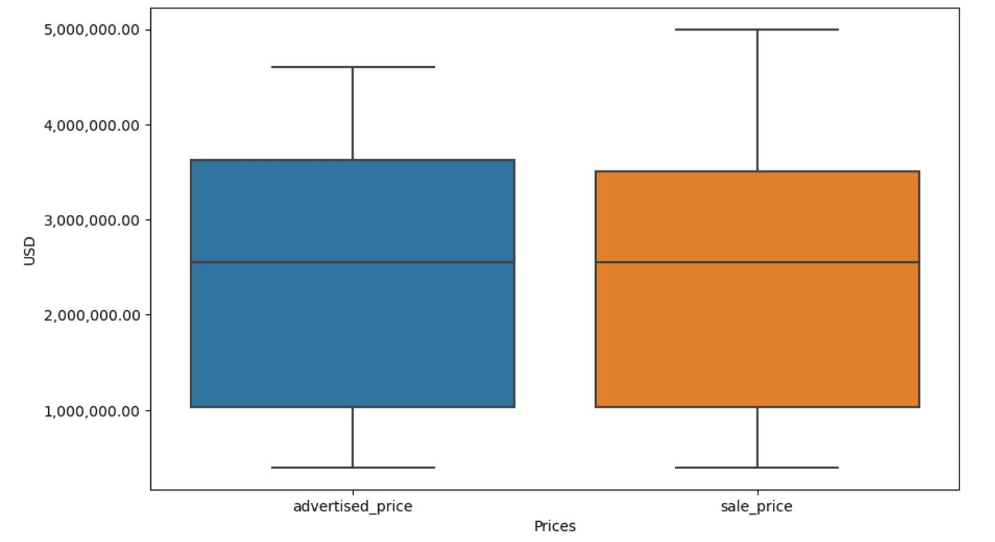
In our instance, the output would be the similar in each instances. To see how the field plot modified, we have to plot it once more utilizing the identical code as earlier.

plt.determine(figsize=(10, 6))
sns.boxplot(information=df[['advertised_price', 'sale_price']])
plt.xlabel('Costs')
plt.ylabel('USD')
plt.ticklabel_format(model="plain", axis="y")
formatter = ticker.FuncFormatter(lambda x, p: format(x, ',.2f'))
plt.gca().yaxis.set_major_formatter(formatter)

Right here’s the output.

You possibly can apply calculating percentiles in Python by fixing the Normal Meeting interview query.

Knowledge cleansing is an important step within the information evaluation course of. Although it may be time-consuming, it is important to make sure the accuracy of your findings.

Happily, Python’s wealthy ecosystem of libraries makes this course of extra manageable. We discovered find out how to take away pointless rows and columns, reformat information, and cope with lacking values and outliers. These are the same old steps that must be carried out on most any information. Nonetheless, you’ll additionally generally must mix two columns into one, confirm the prevailing information, assign labels to it, or eliminate the white areas.

All that is information cleansing, because it means that you can flip messy, real-world information right into a well-structured dataset that you could analyze with confidence. Simply examine the dataset we began with to the one we ended up with.

For those who don’t see the satisfaction on this consequence and the clear information doesn’t make you surprisingly excited, what on this planet are you doing in information science!?
 

Nate Rosidi is an information scientist and in product technique. He is additionally an adjunct professor educating analytics, and is the founding father of StrataScratch, a platform serving to information scientists put together for his or her interviews with actual interview questions from high corporations. Join with him on Twitter: StrataScratch or LinkedIn.